trace_physical_vs_genomic_distance
Reliability status: stable
trace_physical_vs_genomic_distance.py summarizes how physical chromatin-trace distances change with genomic separation. It reads a chromatin trace table, computes pairwise distances between all barcode loci in each trace, bins those distances by genomic distance, and writes a CSV table that can also be plotted as a log-log physical-vs-genomic-distance curve.
The script loads an input trace table supported by ChromatinTraceTable (.ecsv, .dat, .4dn, or .csv).
Each trace is converted into a NumPy array with one row per trace, one column per barcode, and X/Y/Z coordinates in the final dimension.
Genomic separation is computed from barcode## Description midpoint positions, using (Chrom_Start + Chrom_End) / 2, and is reported in kilobase pairs (kbp).
Physical pairwise distances are computed for: - full 3D Euclidean distance, unless –no_3d is used; - projected X-axis distance; - projected Y-axis distance; - projected Z-axis distance.
Physical distances above –dist_threshold are replaced by NaN before summarization.
Genomic distances are split into –gen_dist_bins equally spaced bins, and the median physical distance is reported for each bin and axis.
usage: trace_physical_vs_genomic_distance [-h] --input INPUT
                                          [--data_output DATA_OUTPUT]
                                          [--interloci_output INTERLOCI_OUTPUT]
                                          [-O OUTPUT]
                                          [--output_format {png,svg,pdf}]
                                          [--gen_dist_bins GEN_DIST_BINS]
                                          [--dist_threshold DIST_THRESHOLD]
                                          [--experiment EXPERIMENT] [--no_3d]
                                          [--quiet]
Named Arguments
- --input
Input chromatin trace table (.ecsv, .dat, .4dn, or .csv).
- --data_output
Output CSV for binned physical-vs-genomic distances.
Default:
'binned_physical_vs_genomic_distances.csv'- --interloci_output
Optional CSV for consecutive-locus genomic distances.
- -O, --output
Output filename for the log-log distance plot.
Default:
'_physical_vs_genomic_plot'- --output_format
Possible choices: png, svg, pdf
Output image format. Default = png.
Default:
'png'- --gen_dist_bins
Number of genomic-distance bins. Default: 50
Default:
50- --dist_threshold
Maximum physical distance retained before replacing with NaN. Default: infinity
Default:
numpy.inf- --experiment
Experiment or replicate label to include in the output CSV.
- --no_3d
Only calculate X, Y, and Z axis distances.
Default:
False- --quiet
Disable progress bars.
Default:
False
Output Files
For each trace file analyzed, the script generates:
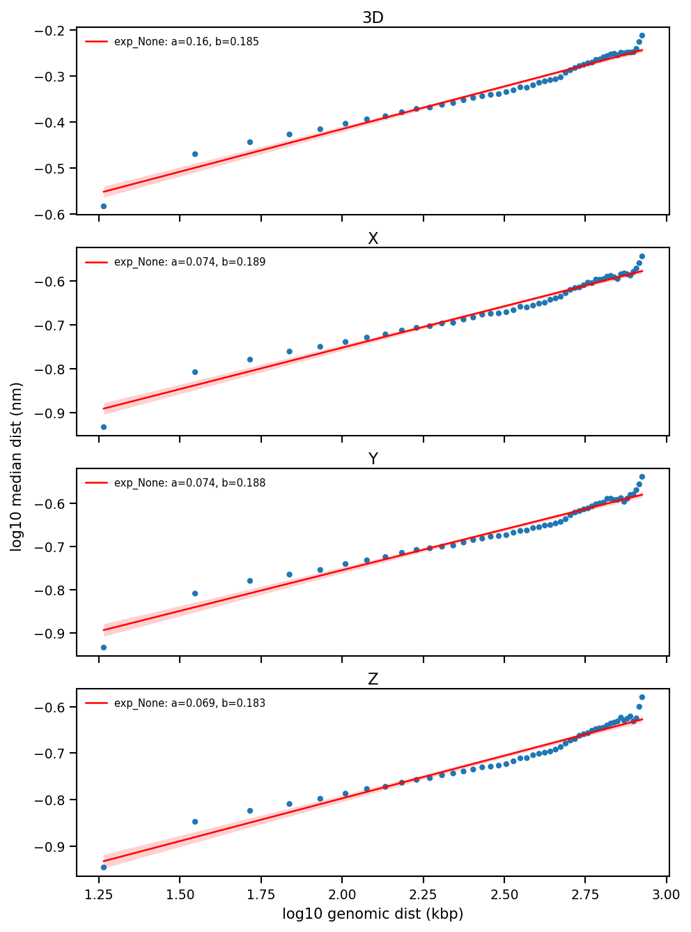
[data_output].csv: CSV file containing one row per genomic-distance bin and axis. The filename comes from--data_output.[interloci_output].csv: Optional CSV file containing genomic distances between consecutive barcode loci. This file is written only when--interloci_outputis provided.[output].[output_format]: Figure with the physical-versus-genomic distance plot, power-law fit, and confidence intervals. The plot path comes from--output/-O(default:_physical_vs_genomic_plot) and the image extension comes from--output_format(default:png). Suffix-style relative output names that start with_are appended to the input trace-file stem.
Examples
trace_physical_vs_genomic_distance.py \
  --input traces_KC_AB_merged.ecsv \
  --data_output binned_physical_vs_genomic_distances.csv \
  --interloci_output interloci_genomic_distances.csv \
  --output _physical_vs_genomic_plot \
  --output_format svg \
  --gen_dist_bins 50 \
  --dist_threshold 1000 \
  --experiment KC_AB
The plot filename is appended to the input stem by default. For the example above, the figure is saved as traces_KC_AB_merged_physical_vs_genomic_plot.svg.
Notes
Plot and power-law fit
The script saves a stacked log-log plot with one panel per calculated axis. The x-axis is shared and shown only on the bottom panel, while a single shared y-axis label spans the panels to avoid label overlap.
For every axis panel and experiment, the script fits the binned median distances to a power-law model:
physical_distance = a * genomic_distance^b
The fit is performed by linear regression in log10 space. The plotted fit line is shown together with a 95% confidence interval for the fitted mean response. Each panel legend reports both fitted coefficients:
a: the scale coefficient.b: the power-law exponent.See the command-line reference above for the complete option list.