Tutorial : Merge Multi-ROI Chromatin Trace Data
This tutorial walks through the standard workflow for merging chromatin tracing data from multiple regions of interest (ROIs):
Collect trace files from all ROIs into one folder
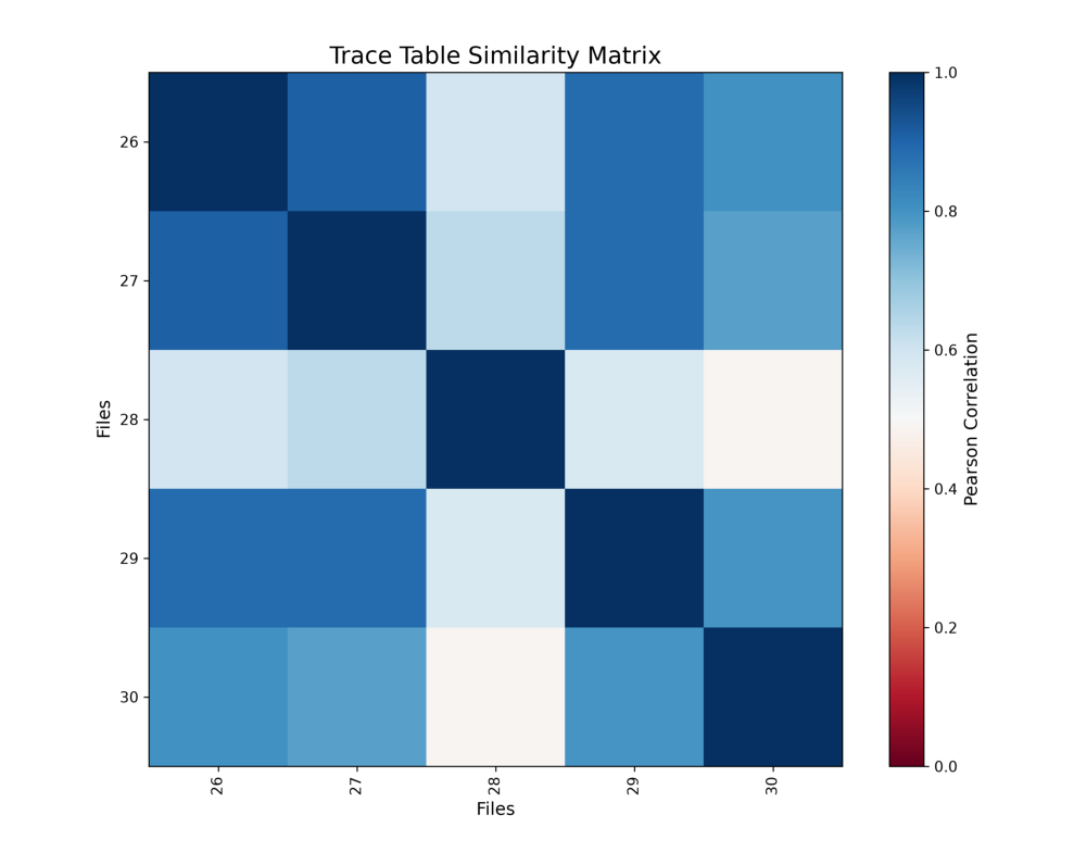
Assess quality by computing Pearson correlations between ROIs
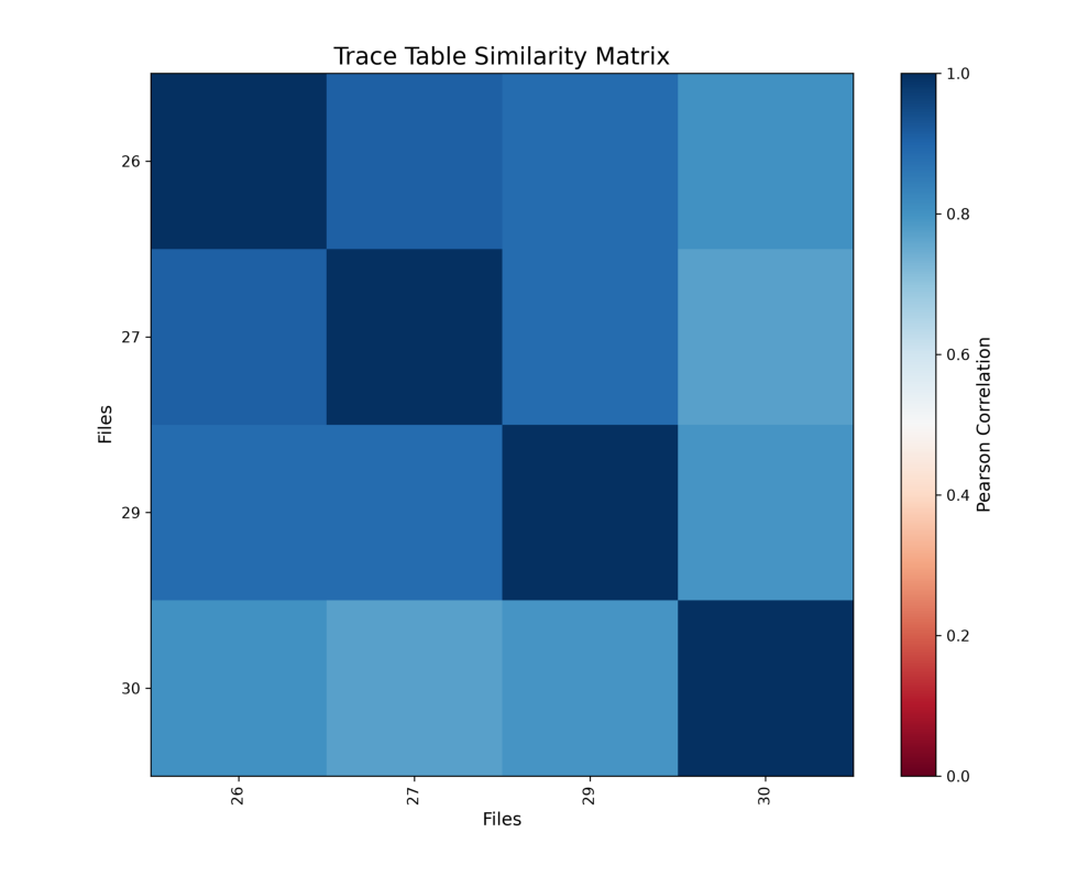
Remove ROIs with poor correlation (outliers)
Re-assess the correlation matrix after removal
Merge the remaining trace files into a single table
Statistics on the merged dataset
Next steps — link to Tutorial 2 for quality control
Step 0: Set-up your data and output path
[1]:
import os
from pathlib import Path
import numpy as np
import matplotlib.pyplot as plt
import matplotlib.image as mpimg
%matplotlib inline
Download datasets from docs/source/…
Set up your folder data path:
[2]:
data_path = "/mnt/grey/DATA/users/zidoum/traceraptops/data/Boettiger/Replicate2"
Set up destination folder for output:
[3]:
dest_path = f"{data_path}/output"
Check ROIs detected:
[4]:
print(f"Data path: {data_path}")
print(f"Output path: {dest_path}")
print(f"\nAvailable ROIs:")
for d in sorted(Path(data_path).iterdir()):
    if d.is_dir() and "FOV" in d.name:
        print(f"  {d.name}")
Data path: /mnt/grey/DATA/users/zidoum/traceraptops/data/Boettiger/Replicate2
Output path: /mnt/grey/DATA/users/zidoum/traceraptops/data/Boettiger/Replicate2/output

Available ROIs:
  FOV_26
  FOV_27
  FOV_28
  FOV_29
  FOV_30
Step 1: Collect trace files from all ROIs
collect_files scans each subdirectory of --root for a file matching --example-file. The --variable-part "13" indicates that the ROI number varies; fixed-length matching naturally excludes Matrix files (different filename length).
[5]:
!collect_files --root {data_path} --example-file "FOV_26_4DNFI2HV38L6.csv" --variable-part "26" --copy-to {dest_path}/raw_traces --force
------- Running collect_files.py --------
Collect one file per subdirectory using pattern matching.

Matched (5):
  FOV_26 -> /mnt/grey/DATA/users/zidoum/traceraptops/data/Boettiger/Replicate2/FOV_26/FOV_26_4DNFI2HV38L6.csv
  FOV_27 -> /mnt/grey/DATA/users/zidoum/traceraptops/data/Boettiger/Replicate2/FOV_27/FOV_27_4DNFI2HV38L6.csv
  FOV_28 -> /mnt/grey/DATA/users/zidoum/traceraptops/data/Boettiger/Replicate2/FOV_28/FOV_28_4DNFI2HV38L6.csv
  FOV_29 -> /mnt/grey/DATA/users/zidoum/traceraptops/data/Boettiger/Replicate2/FOV_29/FOV_29_4DNFI2HV38L6.csv
  FOV_30 -> /mnt/grey/DATA/users/zidoum/traceraptops/data/Boettiger/Replicate2/FOV_30/FOV_30_4DNFI2HV38L6.csv

Copied 5 file(s) to /mnt/grey/DATA/users/zidoum/traceraptops/data/Boettiger/Replicate2/output/raw_traces
Step 2: Compute Pearson correlations between ROIs
trace_pearsons computes a pairwise distance map for each ROI (median 3D distance between every barcode pair), then calculates the Pearson correlation between these maps.
A high correlation between two ROIs means they share similar chromatin organization. An ROI with low correlation against all others is likely an outlier (imaging artifact, poor segmentation, etc.).
[6]:
!ls {dest_path}/raw_traces/*.csv | trace_pearsons --pipe -O {dest_path}

# Display the correlation matrix
img = mpimg.imread(f"{dest_path}/trace_correlation_matrix.png")
fig, ax = plt.subplots(figsize=(10, 10))
ax.imshow(img)
ax.axis('off')
plt.tight_layout()
plt.show()
------- Running trace_pearsons.py --------
Compare chromatin trace tables by computing pairwise distances.

Analyzing 5 trace files...
Processing FOV_26_4DNFI2HV38L6.csv
Processing FOV_27_4DNFI2HV38L6.csv
Processing FOV_28_4DNFI2HV38L6.csv
Processing FOV_29_4DNFI2HV38L6.csv
Processing FOV_30_4DNFI2HV38L6.csv
$ Saved correlation matrix as /mnt/grey/DATA/users/zidoum/traceraptops/data/Boettiger/Replicate2/output/trace_correlation_matrix.png
$ Saved correlation matrix data in NPY format: /mnt/grey/DATA/users/zidoum/traceraptops/data/Boettiger/Replicate2/output/trace_correlation_matrix.npy
Step 4: Re-run Pearson to verify improvement
After removing the outlier ROIs, the correlation matrix should show higher overall values.
[8]:
!ls {dest_path}/raw_traces/*.csv | trace_pearsons --pipe -O {dest_path}

# Display the updated correlation matrix
img = mpimg.imread(f"{dest_path}/trace_correlation_matrix.png")
fig, ax = plt.subplots(figsize=(10, 10))
ax.imshow(img)
ax.axis('off')
plt.tight_layout()
plt.show()
------- Running trace_pearsons.py --------
Compare chromatin trace tables by computing pairwise distances.

Analyzing 4 trace files...
Processing FOV_26_4DNFI2HV38L6.csv
Processing FOV_27_4DNFI2HV38L6.csv
Processing FOV_29_4DNFI2HV38L6.csv
Processing FOV_30_4DNFI2HV38L6.csv
$ Saved correlation matrix as /mnt/grey/DATA/users/zidoum/traceraptops/data/Boettiger/Replicate2/output/trace_correlation_matrix.png
$ Saved correlation matrix data in NPY format: /mnt/grey/DATA/users/zidoum/traceraptops/data/Boettiger/Replicate2/output/trace_correlation_matrix.npy
Step 5: Merge trace files
[9]:
!ls {dest_path}/raw_traces/*.csv | trace_merge -F {dest_path} -N merged_traces.ecsv
------- Running trace_merge.py --------
This script will merge trace tables provided as inputs.

Number of trace files to merge: 4
 $ Merged trace file will contain 94893 traces
Read and accumulated 4 trace files
$ Saving output table as /mnt/grey/DATA/users/zidoum/traceraptops/data/Boettiger/Replicate2/output/merged_traces.ecsv ...
Finished execution
Step 6: Compute basic statistics
[10]:
!trace_stats --input {dest_path}/merged_traces.ecsv
------- Running trace_stats.py --------
Compute basic statistics for chromatin trace files.

$ Importing table from pyHiM format
Successfully loaded trace table: /mnt/grey/DATA/users/zidoum/traceraptops/data/Boettiger/Replicate2/output/merged_traces.ecsv
Statistics for /mnt/grey/DATA/users/zidoum/traceraptops/data/Boettiger/Replicate2/output/merged_traces.ecsv:
- Number of unique ROIs: 4
- Number of unique chromatin traces: 1792
- Number of unique barcodes: 70
Next steps
The merged trace file is ready for downstream analysis.
Continue with Tutorial 2 — Quality Control to:
Generate detailed quality metrics with
trace_analyzerInterpret barcode detection, neighbor distances, and barcode frequency plots
Decide on filtering thresholds for Tutorial 3
Summary
Step |
Script |
Output |
|---|---|---|
Collect |
|
|
Correlations |
|
|
Filter ROIs |
Python (numpy) |
removed outlier files from |
Merge |
|
|
Statistics |
|
stdout |
Output location: data/output/