Tutorial 5: Split Oversized Traces

The Problem

Some traces in the dataset are abnormally large. This happens when the tracing algorithm incorrectly groups multiple chromatin fibers into a single trace. These oversized traces distort downstream distance and contact analyses.

How trace_splitter Works

trace_splitter uses a two-step approach:

1. Measure trace size — Compute the radius of gyration (Rg) of each trace. Rg is the average distance of all barcode positions from the trace’s center of mass:

   Rg = sqrt( mean( |position - center_of_mass|² ) )

   A larger Rg means the trace is more spread out in 3D space.

2. Split large traces — Traces with Rg above a threshold (mean + std_threshold × std) are split into sub-traces using K-means clustering on their 3D coordinates. Each resulting cluster gets a new Trace_ID.

Input

The duplicate-cleaned trace file from Tutorial 4: merged_traces_cleaned_intensity.ecsv

import matplotlib.pyplot as plt
import matplotlib.image as mpimg

data_path = "/mnt/grey/DATA/users/zidoum/traceraptops/jupyterlab_amel"
dest_path = f"{data_path}/output"

input_trace = f"{dest_path}/merged_traces.ecsv"

print(f"Input: {input_trace}")

Input: /mnt/grey/DATA/users/zidoum/traceraptops/jupyterlab_amel/output/merged_traces.ecsv

Step 1: Run QC Before Splitting

First, let’s run trace_analyzer on the input to have a reference for comparison.

!trace_analyzer --input {input_trace}

------- Running trace_analyzer.py --------
Analyze chromatin trace files.


1 trace files to process= /mnt/grey/DATA/users/zidoum/traceraptops/jupyterlab_amel/output/merged_traces.ecsv
$ Importing table from pyHiM format
Successfully loaded trace table: /mnt/grey/DATA/users/zidoum/traceraptops/jupyterlab_amel/output/merged_traces.ecsv
> Analyzing traces for /mnt/grey/DATA/users/zidoum/traceraptops/jupyterlab_amel/output/merged_traces.ecsv
$ Number of spots in trace file: 83031
$ Calculating overall barcode detection across 16777 traces...
$ Exporting barcode detection plot to: /mnt/grey/DATA/users/zidoum/traceraptops/jupyterlab_amel/output/merged_traces_barcode_detection.png
$ Saved neighbor distances plot: /mnt/grey/DATA/users/zidoum/traceraptops/jupyterlab_amel/output/merged_traces_first_neighbor_distances.png
$ Mean distances between neighboring barcodes: X=-0.001, Y=0.000, Z=-0.039
$ Calculating barcode stats...
$ Exporting relative barcode frequencies figure to: /mnt/grey/DATA/users/zidoum/traceraptops/jupyterlab_amel/output/merged_traces_relative_barcode_frequencies.png
$ Saved KDE projection plot: /mnt/grey/DATA/users/zidoum/traceraptops/jupyterlab_amel/output/merged_traces_kde_projections.png
Finished execution

# Display reference plots
before_stats = f"{dest_path}/merged_traces_trace_statistics.png"
before_detect = f"{dest_path}/merged_traces_barcode_detection.png"

fig, axes = plt.subplots(1, 2, figsize=(20, 6))
for ax, f, title in zip(axes, [before_stats, before_detect],
                         ["Trace Statistics (before split)", "Barcode Detection (before split)"]):
    ax.imshow(mpimg.imread(f))
    ax.set_title(title, fontsize=14)
    ax.axis('off')
plt.tight_layout()
plt.show()

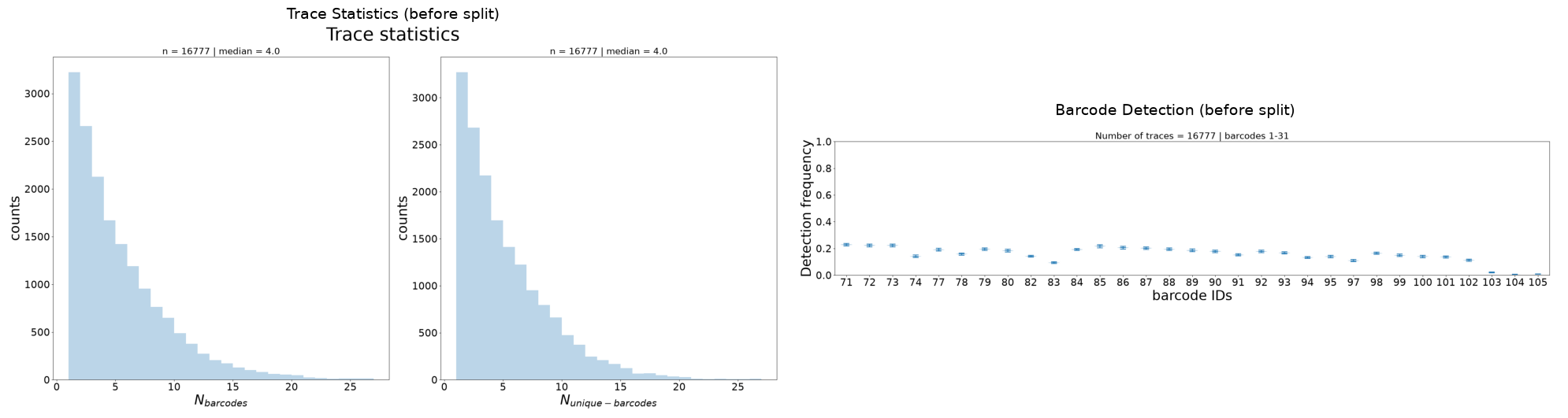
Step 2: Split Oversized Traces

Run trace_splitter with default parameters:

• --std_threshold 1.0 — split traces with Rg > mean + 1×std

• --num_clusters 2 — split each oversized trace into 2 sub-traces

!trace_splitter --input {input_trace}

------- Running trace_splitter.py --------
Split chromatin traces using K-means clustering when radius of gyration exceeds a threshold.


1 trace files to process= /mnt/grey/DATA/users/zidoum/traceraptops/jupyterlab_amel/output/merged_traces.ecsv
$ Importing table from pyHiM format
Successfully loaded trace table: /mnt/grey/DATA/users/zidoum/traceraptops/jupyterlab_amel/output/merged_traces.ecsv
Applying K-means clustering with 2 clusters on traces with Rg > mean + 1.0 * std_dev...
$ Mean Rg: 0.324, Std Rg: 0.354, Threshold: 0.678
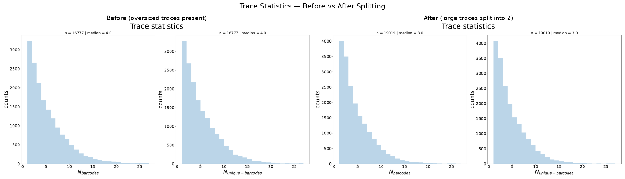
$ Number of traces split: 2242/16777
$ Saving output table as /mnt/grey/DATA/users/zidoum/traceraptops/jupyterlab_amel/output/merged_traces_split.ecsv ...

The output reports:

• The computed Mean Rg, Std Rg, and Threshold

• Each trace that was split, with its Rg value

• Total number of traces split vs total

The output file is saved as <input>_split.ecsv alongside the input.

Step 3: Compare Before vs After

Run trace_analyzer on the split output and compare the trace statistics.

split_trace = f"{dest_path}/merged_traces_split.ecsv"
!trace_analyzer --input {split_trace}

------- Running trace_analyzer.py --------
Analyze chromatin trace files.


1 trace files to process= /mnt/grey/DATA/users/zidoum/traceraptops/jupyterlab_amel/output/merged_traces_split.ecsv
$ Importing table from pyHiM format
Successfully loaded trace table: /mnt/grey/DATA/users/zidoum/traceraptops/jupyterlab_amel/output/merged_traces_split.ecsv
> Analyzing traces for /mnt/grey/DATA/users/zidoum/traceraptops/jupyterlab_amel/output/merged_traces_split.ecsv
$ Number of spots in trace file: 83031
$ Calculating overall barcode detection across 19019 traces...
$ Exporting barcode detection plot to: /mnt/grey/DATA/users/zidoum/traceraptops/jupyterlab_amel/output/merged_traces_split_barcode_detection.png
$ Saved neighbor distances plot: /mnt/grey/DATA/users/zidoum/traceraptops/jupyterlab_amel/output/merged_traces_split_first_neighbor_distances.png
$ Mean distances between neighboring barcodes: X=-0.001, Y=-0.000, Z=-0.006
$ Calculating barcode stats...
$ Exporting relative barcode frequencies figure to: /mnt/grey/DATA/users/zidoum/traceraptops/jupyterlab_amel/output/merged_traces_split_relative_barcode_frequencies.png
$ Saved KDE projection plot: /mnt/grey/DATA/users/zidoum/traceraptops/jupyterlab_amel/output/merged_traces_split_kde_projections.png
Finished execution

# Compare: Trace Statistics before vs after
after_stats = f"{dest_path}/merged_traces_split_trace_statistics.png"

fig, axes = plt.subplots(1, 2, figsize=(20, 6))
for ax, f, title in zip(axes, [before_stats, after_stats],
                         ["Before (oversized traces present)",
                          "After (large traces split into 2)"]):
    ax.imshow(mpimg.imread(f))
    ax.set_title(title, fontsize=14)
    ax.axis('off')
fig.suptitle("Trace Statistics — Before vs After Splitting", fontsize=16)
plt.tight_layout()
plt.show()

# Compare: Barcode Detection before vs after
after_detect = f"{dest_path}/merged_traces_split_barcode_detection.png"

fig, axes = plt.subplots(1, 2, figsize=(20, 6))
for ax, f, title in zip(axes, [before_detect, after_detect],
                         ["Before", "After splitting"]):
    ax.imshow(mpimg.imread(f))
    ax.set_title(title, fontsize=14)
    ax.axis('off')
fig.suptitle("Barcode Detection — Before vs After Splitting", fontsize=16)
plt.tight_layout()
plt.show()

What to check:

• N_barcodes (left panel) shifts left: split traces have fewer barcodes each

• Total trace count increases: each split creates one extra trace

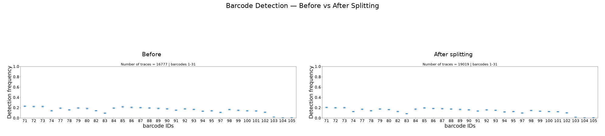
• Barcode detection may change slightly as trace composition is modified

About the Parameters

trace_splitter accepts two parameters with sensible defaults:

Parameter	Default	Effect
--std_threshold	1.0	Traces with Rg > mean + N×std are split. Lower = more aggressive.
--num_clusters	2	Number of sub-traces after splitting.

The defaults are recommended for most datasets. Changing them requires a good reason:

• Lowering --std_threshold (e.g. 0.5) splits more traces, risking splitting legitimate extended conformations

• Raising --std_threshold (e.g. 2.0) only splits extreme outliers

• --num_clusters 3 would only make sense if you suspect three distinct fibers were merged into a single trace, which is rare

When in doubt, keep the defaults and inspect the results.

Summary

What	How
Detect oversized traces	Radius of gyration (Rg) > mean + std
Split them	K-means clustering on 3D coordinates
Default behavior	Split into 2, threshold at mean + 1×std

trace_splitter only modifies traces above the Rg threshold. All other traces pass through unchanged.

Next: Tutorial 6 — Assign Masks & Split by Labels