Tutorial 9: Compare Datasets

Objective

Quantitatively compare chromatin organization between two experimental conditions. In this tutorial we compare traces from Pdx1-positive cells (inside the Pdx1 mask) versus Pdx1-negative cells (outside the mask), using the split files from Tutorial 6 and the PWD matrices computed in Tutorial 7.

Two complementary scripts are covered:

1. ``plot_matrix_comparison`` — Pearson correlation scatter plot + violin distribution comparison (with Wilcoxon rank-sum p-value).

2. ``plot_compare2matrices`` — Side-by-side matrix visualizations: difference matrix, mixed matrix (upper/lower triangle), and Wilcoxon statistical-test matrix.

Scientific context

• Pearson scatter: quantifies overall similarity between two distance/proximity matrices. r ≈ 1 means highly similar; r ≈ 0 means largely uncorrelated.

• Violin plot: compares the full distribution of pairwise values between the two conditions (Wilcoxon rank-sum test for significance).

• Difference matrix: highlights which barcode pairs change the most between conditions.

• Mixed matrix: upper triangle = condition 1, lower triangle = condition 2 — visual comparison on a single heatmap.

• Wilcoxon matrix: per-barcode-pair statistical significance across single-cell measurements.

Input

We use the single-cell PWD matrices produced by trace_to_matrix (Tutorial 7) for each condition:

File	Description
..._Pdx1_Pdx1_Matrix_PWDscMatrix.npy	3D single-cell PWD matrix (Pdx1+)
..._not:Pdx1_Matrix_PWDscMatrix.npy	3D single-cell PWD matrix (Pdx1−)
..._Pdx1_Pdx1_Matrix_uniqueBarcodes.ecsv	Barcode list (shared)

import matplotlib.pyplot as plt
import matplotlib.image as mpimg
import glob

data_path = "/home/devos/Documents/data_to_compare_pdx1/matrix"

# Single-cell PWD matrices (3D: n_barcodes x n_barcodes x n_traces)
matrix_pdx1_pos = f"{data_path}/merged_traces_PDX1_split_Matrix_PWDscMatrix.npy"
matrix_pdx1_neg = f"{data_path}/merged_traces_NOT_PDX1_split_Matrix_PWDscMatrix.npy"

# Unique barcodes (same for both — they come from the same ROI)
barcodes = f"{data_path}/merged_traces_split_Matrix_uniqueBarcodes.ecsv"

print(f"Pdx1+ matrix: {matrix_pdx1_pos}")
print(f"Pdx1- matrix: {matrix_pdx1_neg}")
print(f"Barcodes:     {barcodes}")

Pdx1+ matrix: /home/devos/Documents/data_to_compare_pdx1/matrix/merged_traces_PDX1_split_Matrix_PWDscMatrix.npy
Pdx1- matrix: /home/devos/Documents/data_to_compare_pdx1/matrix/merged_traces_NOT_PDX1_split_Matrix_PWDscMatrix.npy
Barcodes:     /home/devos/Documents/data_to_compare_pdx1/matrix/merged_traces_split_Matrix_uniqueBarcodes.ecsv

Step 1: Pearson correlation with plot_matrix_comparison

plot_matrix_comparison takes two single-cell PWD matrices, computes ensemble averages (median, KDE, or proximity), flattens the upper triangle into vectors, and:

1. Computes the Pearson correlation between the two vectors.

2. Produces a scatter plot (dataset 1 vs dataset 2) with the identity line.

3. Produces a violin plot comparing the distributions (with Wilcoxon p-value).

Parameters

Option	Default	Description
--input1	—	First single-cell PWD matrix (.npy)
--input2	—	Second single-cell PWD matrix (.npy)
--output	output.png	Base name for output plots
--mode	median	Averaging method: median, KDE, or proximity
--scale	linear	Axis scale: linear or log
--max_distance	inf	Upper distance threshold (µm)

# Pearson correlation using median distances
!plot_matrix_comparison --input1 {matrix_pdx1_pos} --input2 {matrix_pdx1_neg} --mode median --output {data_path}/comparison_median.png

Input parameters
================
input1-->/home/devos/Documents/data_to_compare_pdx1/matrix/merged_traces_PDX1_split_Matrix_PWDscMatrix.npy
input2-->/home/devos/Documents/data_to_compare_pdx1/matrix/merged_traces_NOT_PDX1_split_Matrix_PWDscMatrix.npy
output-->/home/devos/Documents/data_to_compare_pdx1/matrix/comparison_median.png
mode-->median
x_min-->None
x_max-->None
max_distance-->inf
scale-->linear
input_files-->['/home/devos/Documents/data_to_compare_pdx1/matrix/merged_traces_PDX1_split_Matrix_PWDscMatrix.npy', '/home/devos/Documents/data_to_compare_pdx1/matrix/merged_traces_NOT_PDX1_split_Matrix_PWDscMatrix.npy']
> Number of input files: 2
Input files:
/home/devos/Documents/data_to_compare_pdx1/matrix/merged_traces_PDX1_split_Matrix_PWDscMatrix.npy
/home/devos/Documents/data_to_compare_pdx1/matrix/merged_traces_NOT_PDX1_split_Matrix_PWDscMatrix.npy
--------------------------------------------------------------------------------
Processing files
================
/home/devos/Repo/traceratops/.venv/lib/python3.11/site-packages/numpy/lib/_nanfunctions_impl.py:1215: RuntimeWarning: All-NaN slice encountered
  return fnb._ureduce(a, func=_nanmedian, keepdims=keepdims,
$ Converted 23x23 matrix to vector of length: 253
$ Converted 23x23 matrix to vector of length: 253
> Output image saved as : /home/devos/Documents/data_to_compare_pdx1/matrix/comparison_median_violin_plot.png
Pearson Correlation Coefficient:  0.9676919891487606
$ limits: 0.19999314844608307-->0.39745526015758514
> Output image saved as : /home/devos/Documents/data_to_compare_pdx1/matrix/comparison_median_scatter_plot.png
Finished execution
--------------------------------------------------------------------------------

This produces two plots:

Output	Description
comparison_median_scatter_plot.png	Scatter plot with Pearson r
comparison_median_violin_plot.png	Violin distributions with Wilcoxon p-value

fig, axes = plt.subplots(1, 2, figsize=(22, 10))

scatter_file = f"{data_path}/comparison_median_scatter_plot.png"
violin_file = f"{data_path}/comparison_median_violin_plot.png"

img_scatter = mpimg.imread(scatter_file)
axes[0].imshow(img_scatter)
axes[0].axis('off')
axes[0].set_title("Pearson correlation (median distances)", fontsize=14)

img_violin = mpimg.imread(violin_file)
axes[1].imshow(img_violin)
axes[1].axis('off')
axes[1].set_title("Distribution comparison (Wilcoxon)", fontsize=14)

plt.tight_layout()
plt.show()

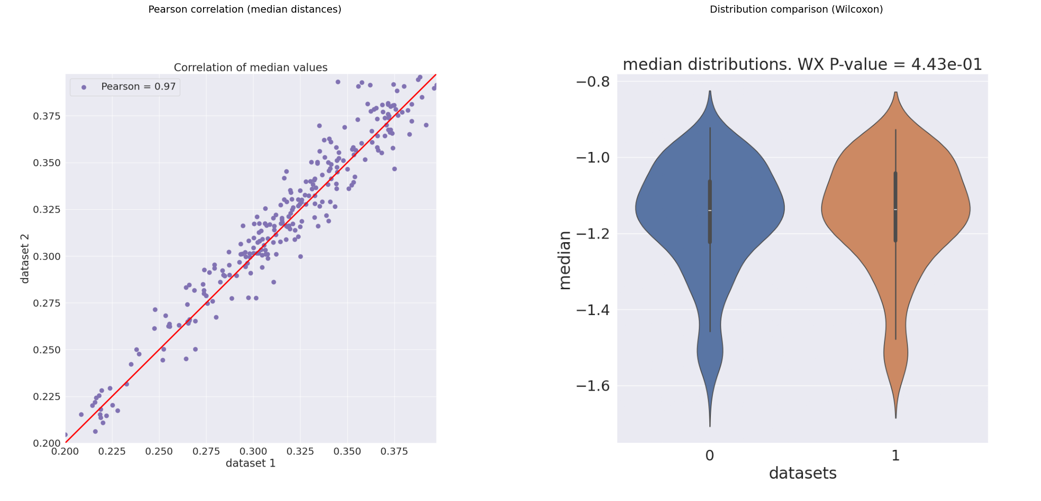
How to read these plots:

• Scatter plot: each point is one barcode pair. Points on the identity line (red) mean identical values in both conditions. The Pearson r is shown in the legend.

• Violin plot: log-transformed distributions of pairwise values for each dataset. The Wilcoxon rank-sum p-value tests whether the two distributions differ significantly.

A high Pearson r (> 0.9) with a non-significant Wilcoxon test suggests the overall chromatin architecture is conserved between conditions.

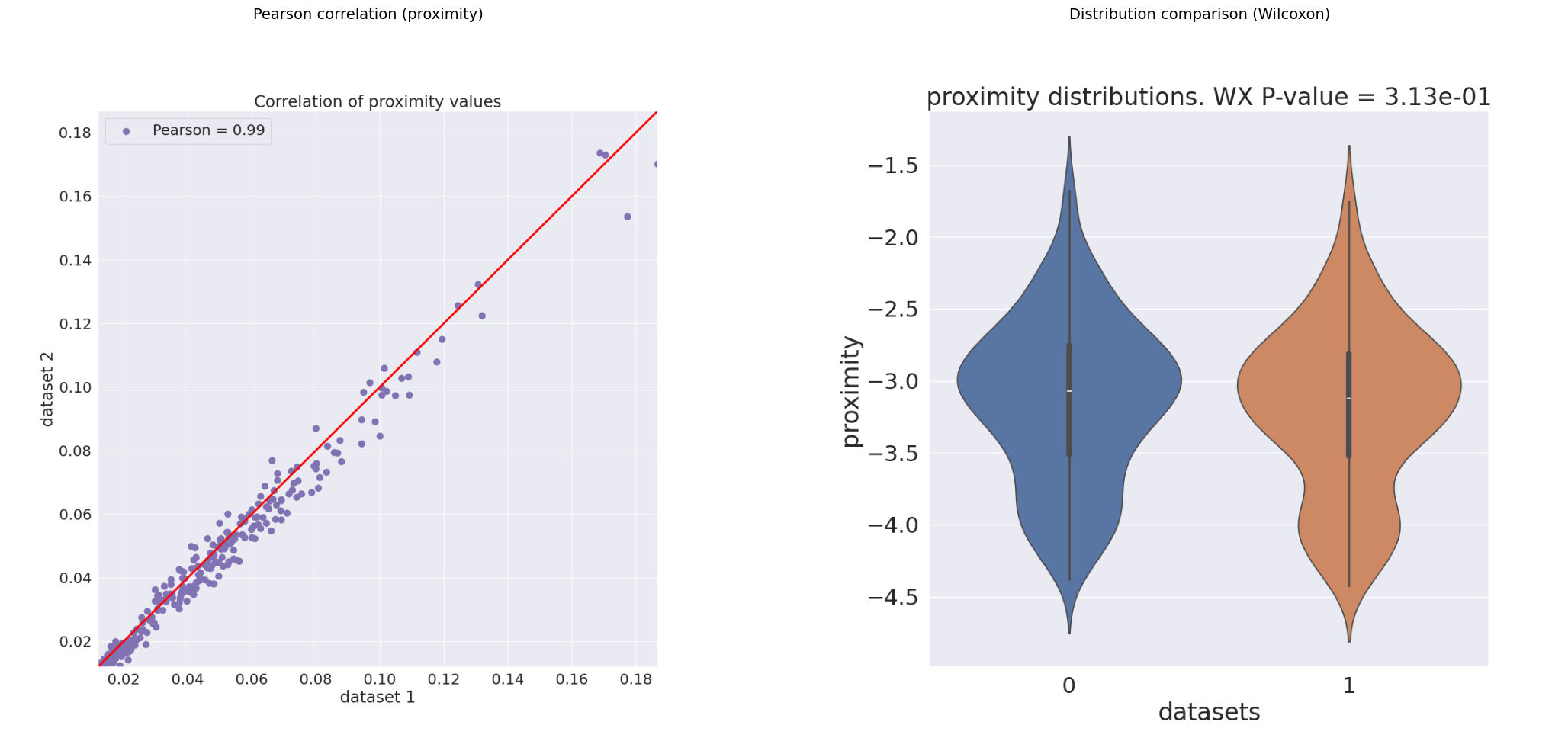
Proximity mode

You can also compare contact probability matrices instead of distances. In proximity mode, the matrix values are the fraction of traces where each barcode pair is within the contact threshold.

# Pearson correlation using contact proximity
!plot_matrix_comparison --input1 {matrix_pdx1_pos} --input2 {matrix_pdx1_neg} --mode proximity --output {data_path}/comparison_proximity.png

Input parameters
================
input1-->/home/devos/Documents/data_to_compare_pdx1/matrix/merged_traces_PDX1_split_Matrix_PWDscMatrix.npy
input2-->/home/devos/Documents/data_to_compare_pdx1/matrix/merged_traces_NOT_PDX1_split_Matrix_PWDscMatrix.npy
output-->/home/devos/Documents/data_to_compare_pdx1/matrix/comparison_proximity.png
mode-->proximity
x_min-->None
x_max-->None
max_distance-->inf
scale-->linear
input_files-->['/home/devos/Documents/data_to_compare_pdx1/matrix/merged_traces_PDX1_split_Matrix_PWDscMatrix.npy', '/home/devos/Documents/data_to_compare_pdx1/matrix/merged_traces_NOT_PDX1_split_Matrix_PWDscMatrix.npy']
> Number of input files: 2
Input files:
/home/devos/Documents/data_to_compare_pdx1/matrix/merged_traces_PDX1_split_Matrix_PWDscMatrix.npy
/home/devos/Documents/data_to_compare_pdx1/matrix/merged_traces_NOT_PDX1_split_Matrix_PWDscMatrix.npy
--------------------------------------------------------------------------------
Processing files
================
$ Converted 23x23 matrix to vector of length: 253
$ Converted 23x23 matrix to vector of length: 253
> Output image saved as : /home/devos/Documents/data_to_compare_pdx1/matrix/comparison_proximity_violin_plot.png
Pearson Correlation Coefficient:  0.9885946081825399
$ limits: 0.011965811965811967-->0.1867816091954023
> Output image saved as : /home/devos/Documents/data_to_compare_pdx1/matrix/comparison_proximity_scatter_plot.png
Finished execution
--------------------------------------------------------------------------------

fig, axes = plt.subplots(1, 2, figsize=(22, 10))

scatter_file = f"{data_path}/comparison_proximity_scatter_plot.png"
violin_file = f"{data_path}/comparison_proximity_violin_plot.png"

img_scatter = mpimg.imread(scatter_file)
axes[0].imshow(img_scatter)
axes[0].axis('off')
axes[0].set_title("Pearson correlation (proximity)", fontsize=14)

img_violin = mpimg.imread(violin_file)
axes[1].imshow(img_violin)
axes[1].axis('off')
axes[1].set_title("Distribution comparison (Wilcoxon)", fontsize=14)

plt.tight_layout()
plt.show()

Step 2: Matrix-level comparison with plot_compare2matrices

plot_compare2matrices produces three publication-quality visualizations that compare two Hi-M matrices element by element:

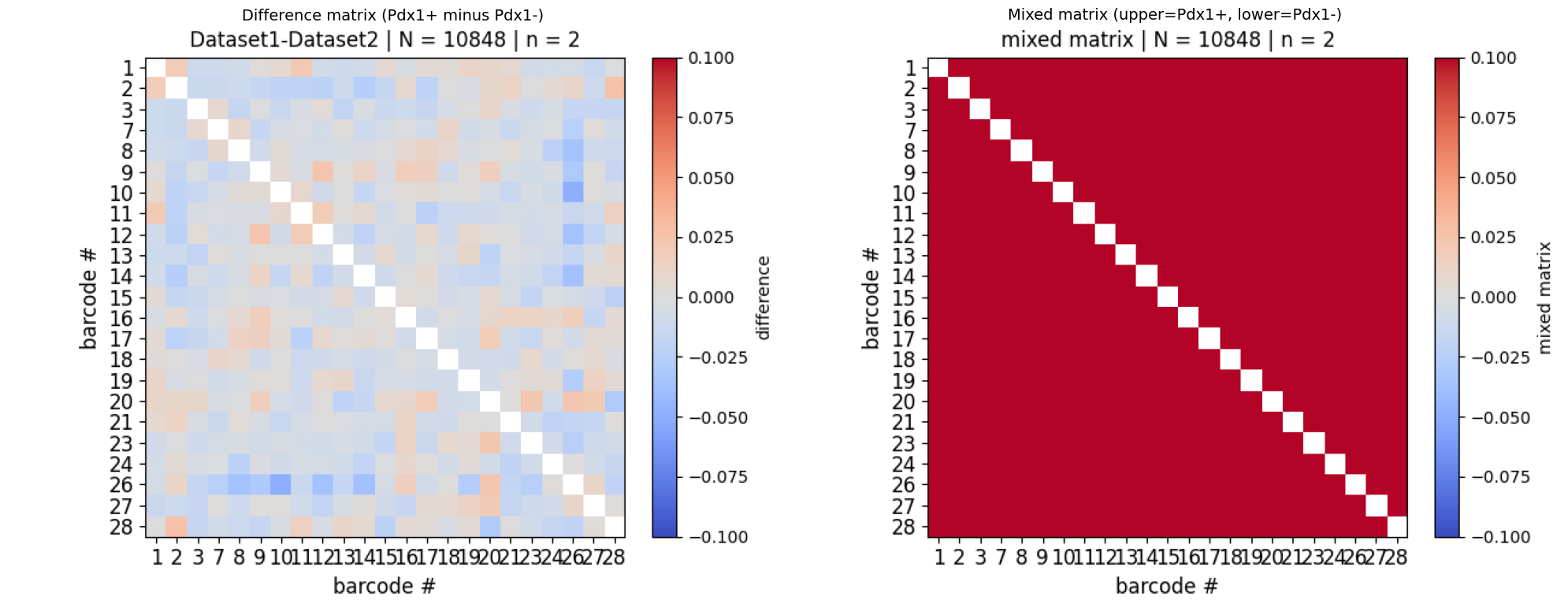
1. Difference matrix — subtracts matrix 2 from matrix 1 (or computes the ratio). Highlights which barcode pairs change the most.

2. Mixed matrix — upper triangle from matrix 1, lower triangle from matrix 2. Allows direct visual comparison on a single heatmap.

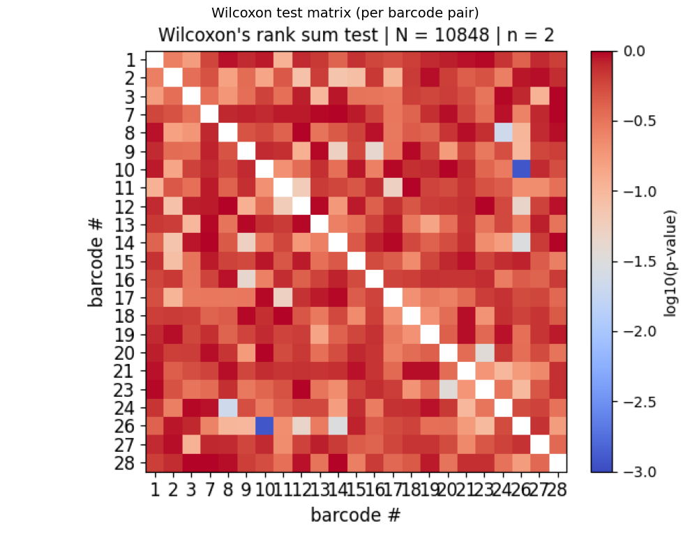
3. Wilcoxon matrix — per-barcode-pair Wilcoxon test across single-cell measurements. Shows which pairs have statistically significant differences. (Only for median/KDE mode.)

Parameters

Option	Default	Description
-T1 / --input1	—	First single-cell PWD matrix (.npy)
-T2 / --input2	—	Second single-cell PWD matrix (.npy)
-U / --uniqueBarcodes	—	Unique barcodes file (.ecsv)
-O / --outputFolder	plots	Output folder
--dist_calc_mode	median	Averaging: median, KDE, or proximity
--ratio	off	Compute ratio instead of difference
--normalize	none	Normalization: maximum, none, or a numeric value
--proximity_threshold	0.25	Contact threshold in µm (for proximity mode)
--cmap	coolwarm	Colormap
--plottingFileExtension	svg	Output format: svg, pdf, or png

# Compare matrices using median distances (produces difference, mixed, and Wilcoxon plots)
!plot_compare2matrices -T1 {matrix_pdx1_pos} -T2 {matrix_pdx1_neg} -U {barcodes} --dist_calc_mode median --plottingFileExtension png -O {data_path}/comparison_plots

Input parameters:{'input1': '/home/devos/Documents/data_to_compare_pdx1/matrix/merged_traces_PDX1_split_Matrix_PWDscMatrix.npy', 'input2': '/home/devos/Documents/data_to_compare_pdx1/matrix/merged_traces_NOT_PDX1_split_Matrix_PWDscMatrix.npy', 'uniqueBarcodes': '/home/devos/Documents/data_to_compare_pdx1/matrix/merged_traces_split_Matrix_uniqueBarcodes.ecsv', 'outputFolder': '/home/devos/Documents/data_to_compare_pdx1/matrix/comparison_plots', 'proximity_threshold': 0.25, 'cmap': 'coolwarm', 'fontsize': 12, 'pixelSize': 1, 'axisLabel': True, 'axisTicks': True, 'ratio': False, 'plottingFileExtension': '.png', 'normalize': 'none', 'dist_calc_mode': 'median', 'cmtitle': 'distance, um', 'matrix_norm_mode': 'n_cells', 'cMax': 0.0, 'scalingParameter': 1, 'shuffle': 0, 'cMin': 0.0}
**************************************************
Folder created: /home/devos/Documents/data_to_compare_pdx1/matrix/comparison_plots
$ Loaded: /home/devos/Documents/data_to_compare_pdx1/matrix/merged_traces_PDX1_split_Matrix_PWDscMatrix.npy
$ N traces to plot: 3828/3828
$ unique barcodes loaded: [1, 2, 3, 7, 8, 9, 10, 11, 12, 13, 14, 15, 16, 17, 18, 19, 20, 21, 23, 24, 26, 27, 28]
$ averaging method: median
$ loaded cScale: 1 | used cScale: 6.943127155303955
/home/devos/Repo/traceratops/.venv/lib/python3.11/site-packages/numpy/lib/_nanfunctions_impl.py:1215: RuntimeWarning: All-NaN slice encountered
  return fnb._ureduce(a, func=_nanmedian, keepdims=keepdims,
--------------------------------------------------
$ Loaded: /home/devos/Documents/data_to_compare_pdx1/matrix/merged_traces_NOT_PDX1_split_Matrix_PWDscMatrix.npy
$ N traces to plot: 7020/7020
$ unique barcodes loaded: [1, 2, 3, 7, 8, 9, 10, 11, 12, 13, 14, 15, 16, 17, 18, 19, 20, 21, 23, 24, 26, 27, 28]
$ averaging method: median
$ loaded cScale: 1 | used cScale: 8.290925979614258
/home/devos/Repo/traceratops/.venv/lib/python3.11/site-packages/numpy/lib/_nanfunctions_impl.py:1215: RuntimeWarning: All-NaN slice encountered
  return fnb._ureduce(a, func=_nanmedian, keepdims=keepdims,
$ Normalization: maximum
Normalizations: m1= 1.0 | m2=0.9958858042908253
$ max_m1 = 0.39745526015758514   max_m2 = 0.39745526015758514
$ calculating difference
$ Clim used: 0.0

barcodes:[1, 2, 3, 7, 8, 9, 10, 11, 12, 13, 14, 15, 16, 17, 18, 19, 20, 21, 23, 24, 26, 27, 28]
Output figure: /home/devos/Documents/data_to_compare_pdx1/matrix/comparison_plots/Fig_merged_traces_PDX1_split_Matrix_PWDscMatrix
$ Normalization: none
Normalizations: m1= 1 | m2=1
$ max_m1 = 0.39745526015758514   max_m2 = 0.3958200514316559
barcodes:[1, 2, 3, 7, 8, 9, 10, 11, 12, 13, 14, 15, 16, 17, 18, 19, 20, 21, 23, 24, 26, 27, 28]
Output figure: /home/devos/Documents/data_to_compare_pdx1/matrix/comparison_plots/Fig_merged_traces_PDX1_split_Matrix_PWDscMatrix_mixed_matrix.png
$ Normalization: none
Normalizations: m1= 1 | m2=1
$ normalization factor: 1
$ max_m1 = 6.943127155303955     max_m2 = 8.290925979614258
/home/devos/Repo/traceratops/traceratops/core/plotting_functions.py:195: RuntimeWarning: divide by zero encountered in log10
  result = np.log10(result)
barcodes:[1, 2, 3, 7, 8, 9, 10, 11, 12, 13, 14, 15, 16, 17, 18, 19, 20, 21, 23, 24, 26, 27, 28]
$ Output figure: /home/devos/Documents/data_to_compare_pdx1/matrix/comparison_plots/Fig_merged_traces_PDX1_split_Matrix_PWDscMatrix_Wilcoxon.png
$ Output data: /home/devos/Documents/data_to_compare_pdx1/matrix/comparison_plots/Fig_merged_traces_PDX1_split_Matrix_PWDscMatrix_Wilcoxon.npy

This produces three plots in the output folder:

Output	Description
*_difference.png	Difference heatmap (matrix 1 − matrix 2)
*_mixed_matrix.png	Upper triangle = Pdx1+, lower = Pdx1−
*_Wilcoxon.png	Per-pair Wilcoxon p-value heatmap

plots_dir = f"{data_path}/comparison_plots"

# Find the generated plots
diff_matches = sorted(glob.glob(f"{plots_dir}/*_difference.png"))
mixed_matches = sorted(glob.glob(f"{plots_dir}/*_mixed_matrix.png"))
wilcoxon_matches = sorted(glob.glob(f"{plots_dir}/*_Wilcoxon.png"))

if diff_matches and mixed_matches:
    fig, axes = plt.subplots(1, 2, figsize=(20, 8))

    img = mpimg.imread(diff_matches[0])
    axes[0].imshow(img)
    axes[0].axis('off')
    axes[0].set_title("Difference matrix (Pdx1+ minus Pdx1-)", fontsize=14)

    img = mpimg.imread(mixed_matches[0])
    axes[1].imshow(img)
    axes[1].axis('off')
    axes[1].set_title("Mixed matrix (upper=Pdx1+, lower=Pdx1-)", fontsize=14)

    plt.tight_layout()
    plt.show()

if wilcoxon_matches:
    img = mpimg.imread(wilcoxon_matches[0])
    fig, ax = plt.subplots(figsize=(10, 8))
    ax.imshow(img)
    ax.axis('off')
    ax.set_title("Wilcoxon test matrix (per barcode pair)", fontsize=14)
    plt.tight_layout()
    plt.show()

How to read these plots:

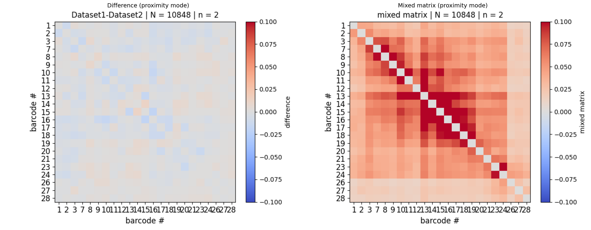
• Difference matrix: warm colors indicate barcode pairs that are closer (or more frequent) in Pdx1+ than Pdx1−, and vice versa for cool colors. Values near zero (white) mean no difference.

• Mixed matrix: the upper triangle shows Pdx1+ and the lower triangle shows Pdx1− on the same color scale. Asymmetries across the diagonal reveal condition-specific contacts.

• Wilcoxon matrix: each cell shows the p-value from a per-barcode-pair Wilcoxon rank-sum test on single-cell distance measurements. Low p-values (dark) indicate pairs where the distance distributions differ significantly between conditions.

Proximity mode comparison

You can also compare contact probability matrices. Note that in proximity mode, the Wilcoxon per-pair matrix is not computed (it requires single-cell distance distributions).

# Compare matrices using contact proximity
!plot_compare2matrices -T1 {matrix_pdx1_pos} -T2 {matrix_pdx1_neg} -U {barcodes} --dist_calc_mode proximity --plottingFileExtension png -O {data_path}/comparison_plots_proximity

Input parameters:{'input1': '/home/devos/Documents/data_to_compare_pdx1/matrix/merged_traces_PDX1_split_Matrix_PWDscMatrix.npy', 'input2': '/home/devos/Documents/data_to_compare_pdx1/matrix/merged_traces_NOT_PDX1_split_Matrix_PWDscMatrix.npy', 'uniqueBarcodes': '/home/devos/Documents/data_to_compare_pdx1/matrix/merged_traces_split_Matrix_uniqueBarcodes.ecsv', 'outputFolder': '/home/devos/Documents/data_to_compare_pdx1/matrix/comparison_plots_proximity', 'proximity_threshold': 0.25, 'cmap': 'coolwarm', 'fontsize': 12, 'pixelSize': 1, 'axisLabel': True, 'axisTicks': True, 'ratio': False, 'plottingFileExtension': '.png', 'normalize': 'none', 'dist_calc_mode': 'proximity', 'cmtitle': 'proximity frequency', 'matrix_norm_mode': 'n_cells', 'cMax': 0.0, 'scalingParameter': 1, 'shuffle': 0, 'cMin': 0.0}
**************************************************
$ Loaded: /home/devos/Documents/data_to_compare_pdx1/matrix/merged_traces_PDX1_split_Matrix_PWDscMatrix.npy
$ N traces to plot: 3828/3828
$ unique barcodes loaded: [1, 2, 3, 7, 8, 9, 10, 11, 12, 13, 14, 15, 16, 17, 18, 19, 20, 21, 23, 24, 26, 27, 28]
$ averaging method: proximity
$ loaded cScale: 1 | used cScale: 6.943127155303955
$ calculating proximity matrix
--------------------------------------------------
$ Loaded: /home/devos/Documents/data_to_compare_pdx1/matrix/merged_traces_NOT_PDX1_split_Matrix_PWDscMatrix.npy
$ N traces to plot: 7020/7020
$ unique barcodes loaded: [1, 2, 3, 7, 8, 9, 10, 11, 12, 13, 14, 15, 16, 17, 18, 19, 20, 21, 23, 24, 26, 27, 28]
$ averaging method: proximity
$ loaded cScale: 1 | used cScale: 8.290925979614258
$ calculating proximity matrix
$ Normalization: maximum
Normalizations: m1= 1.0 | m2=0.9296778435239974
$ max_m1 = 0.1867816091954023    max_m2 = 0.1867816091954023
$ calculating difference
$ Clim used: 0.0

barcodes:[1, 2, 3, 7, 8, 9, 10, 11, 12, 13, 14, 15, 16, 17, 18, 19, 20, 21, 23, 24, 26, 27, 28]
Output figure: /home/devos/Documents/data_to_compare_pdx1/matrix/comparison_plots_proximity/Fig_merged_traces_PDX1_split_Matrix_PWDscMatrix
$ Normalization: none
Normalizations: m1= 1 | m2=1
$ max_m1 = 0.1867816091954023    max_m2 = 0.17364672364672365
barcodes:[1, 2, 3, 7, 8, 9, 10, 11, 12, 13, 14, 15, 16, 17, 18, 19, 20, 21, 23, 24, 26, 27, 28]
Output figure: /home/devos/Documents/data_to_compare_pdx1/matrix/comparison_plots_proximity/Fig_merged_traces_PDX1_split_Matrix_PWDscMatrix_mixed_matrix.png

plots_dir_prox = f"{data_path}/comparison_plots_proximity"

diff_matches = sorted(glob.glob(f"{plots_dir_prox}/*_difference.png"))
mixed_matches = sorted(glob.glob(f"{plots_dir_prox}/*_mixed_matrix.png"))

if diff_matches and mixed_matches:
    fig, axes = plt.subplots(1, 2, figsize=(20, 8))

    img = mpimg.imread(diff_matches[0])
    axes[0].imshow(img)
    axes[0].axis('off')
    axes[0].set_title("Difference (proximity mode)", fontsize=14)

    img = mpimg.imread(mixed_matches[0])
    axes[1].imshow(img)
    axes[1].axis('off')
    axes[1].set_title("Mixed matrix (proximity mode)", fontsize=14)

    plt.tight_layout()
    plt.show()

Summary

Workflow

condition 1 PWD matrix (.npy)  ──┐
                                  ├─── plot_matrix_comparison    →  scatter + violin
condition 2 PWD matrix (.npy)  ──┤
                                  ├─── plot_compare2matrices     →  difference + mixed + Wilcoxon
unique barcodes (.ecsv)  ────────┘

Commands reference

# Pearson correlation + violin distributions
plot_matrix_comparison --input1 matrix1.npy --input2 matrix2.npy --mode median --output comparison.png

# Difference, mixed, and Wilcoxon matrices
plot_compare2matrices -T1 matrix1.npy -T2 matrix2.npy -U barcodes.ecsv --dist_calc_mode median -O output_folder

Key differences between the two scripts

	plot_matrix_comparison	plot_compare2matrices
Input	Two .npy PWD matrices	Two .npy PWD matrices + barcodes file
Approach	Global (whole matrix → vector)	Element-wise (per barcode pair)
Output	Scatter plot + violin	Difference + mixed + Wilcoxon heatmaps
Best for	Overall similarity assessment	Identifying specific pairs that change

Modes

Mode	What it compares
median	Median pairwise 3D distance per barcode pair
KDE	KDE peak distance per barcode pair
proximity	Contact probability (fraction of traces below threshold)

Notes

• Both matrices must have the same dimensions (same barcode ordering). This is guaranteed when both come from the same ROI split by label.

• The Wilcoxon per-pair matrix is only available in median or KDE mode (not in proximity mode, which produces binary counts rather than distances).

• Use --ratio with plot_compare2matrices to compute the ratio instead of the difference between matrices.

• Output format can be changed with --plottingFileExtension (svg, pdf, png).