Tutorial 6: Assign Mask Labels & Split Traces

Objective

In many chromatin tracing experiments, you want to separate traces based on spatial regions defined by a segmentation mask (e.g. a nuclear marker, a tissue boundary, or an immunofluorescence signal).

This tutorial covers two complementary tools:

``trace_assign_mask`` — reads a 2D mask image and tags each spot in a trace file with a label if its (x, y) position falls inside the mask.
``trace_split_labels`` — splits a labeled trace file into two separate files: spots with the label and spots without it.

When to use this

You have a 2D mask (.tif or .npy) that delineates a region of interest (e.g. a nuclear compartment, a specific cell type marker).
You want to compare chromatin organization inside vs. outside that region.
Typical workflow: assign mask → split → run separate analyses on each population.

Input files

File	Description
`Trace_3D_barcode_mask-mask0_ROI-16.ecsv`	A trace file (already filtered)
`MAX_scan_003_RT23_016_ROI.tif`	A 2D mask image (e.g. MAX projection of an IF channel)

[1]:

import matplotlib.pyplot as plt
import matplotlib.image as mpimg

data_path = "/home/xdevos/Repositories/pyHi-M/traceratops/data/data_to_mask"

input_trace = f"{data_path}/Trace_3D_barcode_mask-mask0_ROI-16.ecsv"
mask_file = f"{data_path}/MAX_scan_003_RT23_016_ROI.tif"

print(f"Trace file: {input_trace}")
print(f"Mask file:  {mask_file}")

Trace file: /home/xdevos/Repositories/pyHi-M/traceratops/data/data_to_mask/Trace_3D_barcode_mask-mask0_ROI-16.ecsv
Mask file:  /home/xdevos/Repositories/pyHi-M/traceratops/data/data_to_mask/MAX_scan_003_RT23_016_ROI.tif

Step 1: Assign mask labels with `trace_assign_mask`

The trace_assign_mask command reads each spot’s (x, y) coordinates, converts them to pixel positions using --pixel_size, and checks whether the corresponding pixel in the mask has a value ≥ 1.

If inside the mask → the label (here Pdx1) is appended to the spot’s label column.
If outside → the label column is left unchanged.

Key parameters

Option	Default	Description
`--input`	—	Input trace file (ECSV)
`--mask_file`	—	2D mask image (`.tif`, `.tiff`, or `.npy`)
`--label`	`"labeled"`	Name to assign to spots inside the mask
`--pixel_size`	`0.1`	Lateral pixel size in microns (must match your imaging setup)

[2]:

!trace_assign_mask --input {input_trace} --mask_file {mask_file} --label Pdx1

==========Started execution==========

1 trace files to process= /home/xdevos/Repositories/pyHi-M/traceratops/data/data_to_mask/Trace_3D_barcode_mask-mask0_ROI-16.ecsv
$ Importing table from pyHiM format
Successfully loaded trace table: /home/xdevos/Repositories/pyHi-M/traceratops/data/data_to_mask/Trace_3D_barcode_mask-mask0_ROI-16.ecsv
$ mask image file read: /home/xdevos/Repositories/pyHi-M/traceratops/data/data_to_mask/MAX_scan_003_RT23_016_ROI.tif

> 2802 trace rows out of 7352 were associated to mask Pdx1. Unique traces: 288
$ Saving output table as /home/xdevos/Repositories/pyHi-M/traceratops/data/data_to_mask/Trace_3D_barcode_mask-mask0_ROI-16_Pdx1.ecsv ...
$ Saved output trace file at: /home/xdevos/Repositories/pyHi-M/traceratops/data/data_to_mask/Trace_3D_barcode_mask-mask0_ROI-16_Pdx1.ecsv
$ mask image file read: /home/xdevos/Repositories/pyHi-M/traceratops/data/data_to_mask/MAX_scan_003_RT23_016_ROI.tif
$ Saved mask assignment plot: /home/xdevos/Repositories/pyHi-M/traceratops/data/data_to_mask/Trace_3D_barcode_mask-mask0_ROI-16_Pdx1_mask_plot.png
=========Finished execution=========

This produces two output files next to the input:

Output	Description
`Trace_3D_barcode_mask-mask0_ROI-16_Pdx1.ecsv`	Trace file with `label` column updated
`Trace_3D_barcode_mask-mask0_ROI-16_Pdx1_mask_plot.png`	Diagnostic plot showing assignment

Step 2: Inspect the mask assignment plot

The diagnostic plot overlays spot positions on the mask image:

Red dots: spots inside the mask (labeled Pdx1)
Cyan dots: spots outside the mask (unlabeled)

[3]:

plot_file = f"{data_path}/Trace_3D_barcode_mask-mask0_ROI-16_Pdx1_mask_plot.png"

img = mpimg.imread(plot_file)
fig, ax = plt.subplots(figsize=(10, 10))
ax.imshow(img)
ax.axis('off')
ax.set_title("Mask Assignment: Pdx1", fontsize=14)
plt.tight_layout()
plt.show()

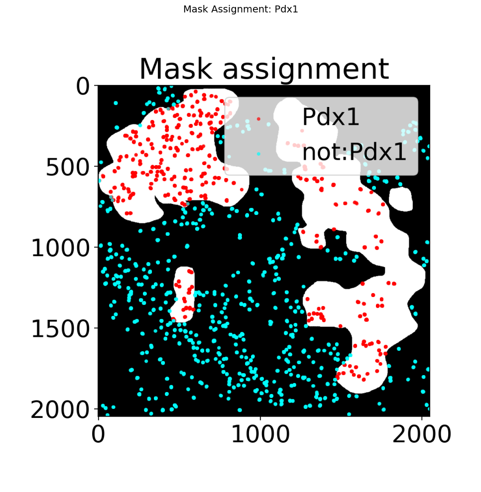
../_images/tutorials_tutorial_06_assign_masks_split_labels_6_0.png

What to check:

Do the red spots align well with the mask boundaries?
If spots appear shifted, verify that --pixel_size matches your microscope calibration.
If spots fall outside the image, the mask dimensions may not match the field of view.

Step 3: Split traces by label with `trace_split_labels`

Now that spots are labeled, use trace_split_labels to separate the trace file into two populations:

Spots with the label (Pdx1) — inside the mask
Spots without the label (not:Pdx1) — outside the mask

This creates two independent ECSV files that can be analyzed separately (e.g. compute Hi-M matrices, barcode statistics, etc.).

[4]:

# Split the labeled trace file
labeled_trace = f"{data_path}/Trace_3D_barcode_mask-mask0_ROI-16_Pdx1.ecsv"

!trace_split_labels --input {labeled_trace} --label Pdx1

========== Started execution ==========

$ Processing 1 trace file(s)

> Processing: /home/xdevos/Repositories/pyHi-M/traceratops/data/data_to_mask/Trace_3D_barcode_mask-mask0_ROI-16_Pdx1.ecsv
$ Importing table from pyHiM format
Successfully loaded trace table: /home/xdevos/Repositories/pyHi-M/traceratops/data/data_to_mask/Trace_3D_barcode_mask-mask0_ROI-16_Pdx1.ecsv
$ Saving output table as /home/xdevos/Repositories/pyHi-M/traceratops/data/data_to_mask/Trace_3D_barcode_mask-mask0_ROI-16_Pdx1_Pdx1.ecsv ...
$ Saving output table as /home/xdevos/Repositories/pyHi-M/traceratops/data/data_to_mask/Trace_3D_barcode_mask-mask0_ROI-16_Pdx1_not:Pdx1.ecsv ...
$ Saved: /home/xdevos/Repositories/pyHi-M/traceratops/data/data_to_mask/Trace_3D_barcode_mask-mask0_ROI-16_Pdx1_Pdx1.ecsv (2802 rows)
$ Saved: /home/xdevos/Repositories/pyHi-M/traceratops/data/data_to_mask/Trace_3D_barcode_mask-mask0_ROI-16_Pdx1_not:Pdx1.ecsv (4550 rows)
========== Finished execution ==========

This produces two files:

Output file	Content
`Trace_3D_barcode_mask-mask0_ROI-16_Pdx1_Pdx1.ecsv`	Spots inside the mask (label contains `Pdx1`)
`Trace_3D_barcode_mask-mask0_ROI-16_Pdx1_not:Pdx1.ecsv`	Spots outside the mask (label does not contain `Pdx1`)

Each file is a valid trace ECSV that can be used directly in downstream analysis pipelines (e.g. trace_to_matrix, plot_him_matrix, trace_analyzer).

Step 4: Verify the split

[5]:

import os

inside_file = f"{data_path}/Trace_3D_barcode_mask-mask0_ROI-16_Pdx1_Pdx1.ecsv"
outside_file = f"{data_path}/Trace_3D_barcode_mask-mask0_ROI-16_Pdx1_not:Pdx1.ecsv"

for name, path in [("Inside mask (Pdx1)", inside_file), ("Outside mask (not:Pdx1)", outside_file)]:
    if os.path.exists(path):
        # Count data lines (skip ECSV header)
        with open(path) as f:
            lines = [l for l in f if not l.startswith('#') and l.strip()]
        n_data = len(lines) - 1  # subtract column header
        print(f"{name}: {n_data} spots  ({os.path.basename(path)})")
    else:
        print(f"{name}: FILE NOT FOUND")

Inside mask (Pdx1): 2802 spots  (Trace_3D_barcode_mask-mask0_ROI-16_Pdx1_Pdx1.ecsv)
Outside mask (not:Pdx1): 4550 spots  (Trace_3D_barcode_mask-mask0_ROI-16_Pdx1_not:Pdx1.ecsv)

Summary

Workflow

trace file + 2D mask
       │
       ▼
trace_assign_mask --label Pdx1     →  labeled trace + diagnostic PNG
       │
       ▼
trace_split_labels --label Pdx1    →  inside.ecsv + outside.ecsv

Commands reference

# 1. Assign mask labels
trace_assign_mask --input Trace.ecsv --mask_file mask.tif --label Pdx1

# 2. Split by label
trace_split_labels --input Trace_Pdx1.ecsv --label Pdx1

Notes

The mask must be 2D (a single plane). If your mask is 3D, take a MAX projection first.
The --pixel_size default is 0.1 µm/pixel. Adjust this if your microscope calibration differs.
You can assign multiple labels by running trace_assign_mask several times with different masks and label names. The labels accumulate in the label column (comma-separated).
trace_split_labels uses string matching: it checks whether the label text appears anywhere in the label column, so it works correctly even with multiple comma-separated labels.

Next: Tutorial 7 — Build Contact Matrices