Tutorial 7: Build and Visualize Hi-M Contact Matrices

Objective

Convert chromatin traces into pairwise distance matrices and contact probability matrices, then visualize them as publication-quality heatmaps.

This tutorial covers two scripts:

1. ``trace_to_matrix`` — computes single-cell pairwise distance (PWD) matrices from a trace file and produces five plots (Hi-M contact matrix, PWD median, PWD KDE, N-matrix, distance histograms).

2. ``plot_him_matrix`` — re-plots a Hi-M matrix from the saved .npy data with custom options (colormap, color range, mode, triangular display, NaN threshold…).

Scientific context

Contact matrices summarize pairwise interactions across all traces:

• Contact probability (Hi-M): fraction of traces where two barcodes are closer than a distance threshold (default 0.25 µm).

• PWD median / KDE: ensemble pairwise distance estimated via median or kernel density peak.

• N-matrix: number of valid (non-NaN) measurements per barcode pair — reveals data coverage.

These matrices reveal chromatin folding patterns such as topologically associating domains (TADs), long-range loops, and compartments.

Input

We use the Pdx1-positive trace file produced by Tutorial 6 (mask assignment + split):

File	Description
Trace_3D_barcode_mask-mask0_ROI-16_Pdx1_Pdx1.ecsv	Traces inside the Pdx1 mask (single ROI)

import matplotlib.pyplot as plt
import matplotlib.image as mpimg

data_path = "/home/devos/Documents/data_to_compare_pdx1/PDX1"

# Pdx1-positive traces from Tutorial 6
input_trace = f"{data_path}/merged_traces_split.ecsv"

# Base name for all matrix outputs
matrix_base = f"{data_path}/merged_traces_split_Matrix"

print(f"Input trace: {input_trace}")

Input trace: /home/devos/Documents/data_to_compare_pdx1/PDX1/merged_traces_split.ecsv

Step 1: Build matrices with trace_to_matrix

trace_to_matrix reads a trace file and computes:

• A 3D single-cell PWD matrix (shape: n_barcodes × n_barcodes × n_traces) saved as .npy

• An N-matrix (count of valid measurements per barcode pair) saved as .npy

• A unique barcodes list saved as .ecsv

• Five plots: Hi-M contact matrix, PWD median, PWD KDE, N-matrix, and distance histograms

Parameters

Option	Default	Description
--input	—	Input trace file (ECSV)
--distance_threshold	inf	Maximum distance allowed (discard pairs beyond this)
-F	./	Output folder (for data files)

!trace_to_matrix --input {input_trace}

$ trace file to process= ['/home/devos/Documents/data_to_compare_pdx1/PDX1/merged_traces_split.ecsv']
$ Importing table from pyHiM format
Successfully loaded trace table: /home/devos/Documents/data_to_compare_pdx1/PDX1/merged_traces_split.ecsv
$ Found 23 barcodes and 3828 traces. INFO
> Processing traces... INFO
100%|██████████████████████████████████████| 3828/3828 [00:05<00:00, 685.76it/s]
100%|███████████████████████████████████████████| 23/23 [00:22<00:00,  1.03it/s]
/home/devos/Repo/traceratops/.venv/lib/python3.11/site-packages/numpy/lib/_nanfunctions_impl.py:1215: RuntimeWarning: All-NaN slice encountered
  return fnb._ureduce(a, func=_nanmedian, keepdims=keepdims,
100%|███████████████████████████████████████████| 23/23 [02:24<00:00,  6.30s/it]
Output figure: /home/devos/Documents/data_to_compare_pdx1/PDX1/merged_traces_split_Matrix_PWDhistograms.png

$ saved: /home/devos/Documents/data_to_compare_pdx1/PDX1/merged_traces_split_Matrix_PWDscMatrix.npy
$ saved: /home/devos/Documents/data_to_compare_pdx1/PDX1/merged_traces_split_Matrix_uniqueBarcodes.ecsv
$ saved: /home/devos/Documents/data_to_compare_pdx1/PDX1/merged_traces_split_Matrix_Nmatrix.npy
Processed <1> trace(s)
Finished execution

Output files

All outputs use the pattern <input_basename>_Matrix_<suffix>:

File	Format	Description
*_Matrix_PWDscMatrix.npy	NumPy binary	3D single-cell pairwise distance matrix
*_Matrix_Nmatrix.npy	NumPy binary	2D N-matrix (data coverage)
*_Matrix_uniqueBarcodes.ecsv	Text	List of unique barcode IDs
*_Matrix_HiMmatrix.png	Image	Contact probability heatmap
*_Matrix_PWDmatrixMedian.png	Image	PWD matrix (median)
*_Matrix_PWDmatrixKDE.png	Image	PWD matrix (KDE peak)
*_Matrix_Nmatrix.png	Image	N-matrix heatmap
*_Matrix_PWDhistograms.png	Image	Distance histograms for all barcode pairs

Step 2: Hi-M contact probability matrix

The Hi-M matrix shows the fraction of traces where each barcode pair is closer than a distance threshold (default: 0.25 µm). Higher values (warm colors) indicate more frequent contacts.

img = mpimg.imread(f"{matrix_base}_HiMmatrix.png")
fig, ax = plt.subplots(figsize=(10, 8))
ax.imshow(img)
ax.axis('off')
ax.set_title("Hi-M Contact Probability Matrix", fontsize=14)
plt.tight_layout()
plt.show()

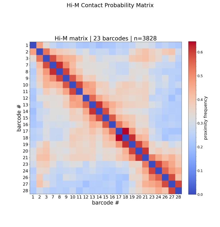
How to read this matrix:

• Axes show barcode IDs (genomic loci along the chromatin fiber).

• The diagonal is always high (a barcode is always close to itself).

• Off-diagonal warm spots indicate frequent spatial proximity between distant genomic loci → potential loops or TAD boundaries.

• Blocks along the diagonal suggest topologically associating domains (TADs).

Step 3: Pairwise distance matrices

Two PWD representations are computed:

• Median: robust central tendency of 3D distances per barcode pair.

• KDE: peak of the kernel density estimate — captures the most probable distance, useful when distributions are skewed.

fig, axes = plt.subplots(1, 2, figsize=(20, 8))

for ax, suffix, title in zip(
    axes,
    ["_PWDmatrixMedian.png", "_PWDmatrixKDE.png"],
    ["PWD Matrix (Median)", "PWD Matrix (KDE)"]
):
    img = mpimg.imread(f"{matrix_base}{suffix}")
    ax.imshow(img)
    ax.axis('off')
    ax.set_title(title, fontsize=14)

plt.tight_layout()
plt.show()

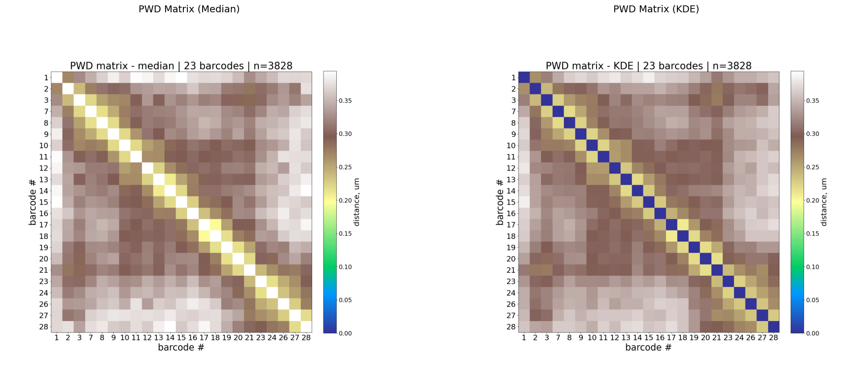
Interpretation:

• Low values along the diagonal (warm colors in terrain colormap) = nearby genomic loci are physically close (expected).

• Off-diagonal low-distance spots indicate long-range contacts.

• KDE is often less noisy than median for sparse data.

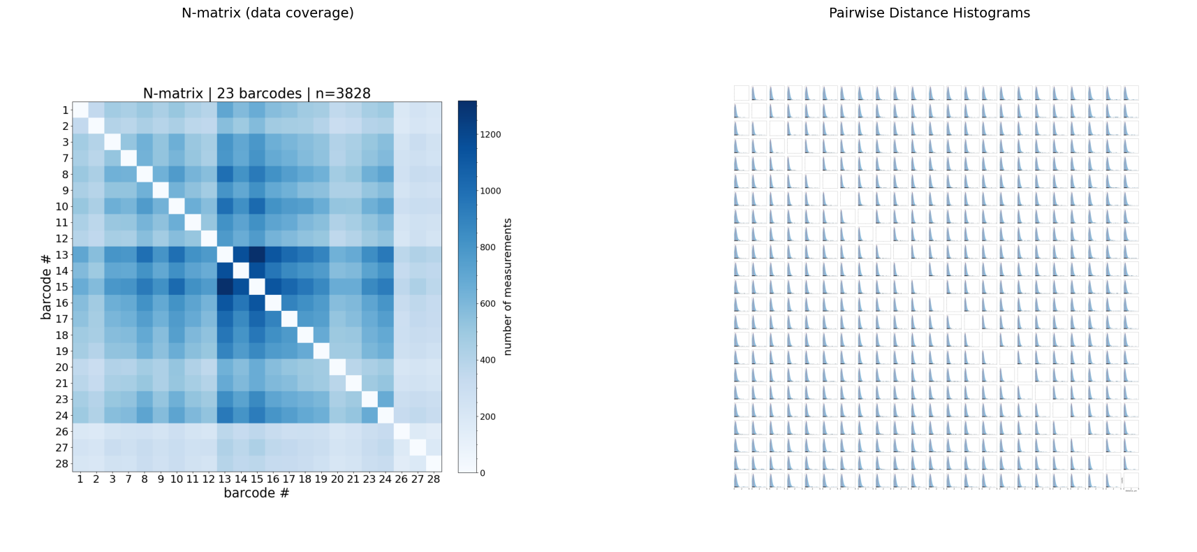
Step 4: N-matrix and distance histograms

The N-matrix shows how many valid (non-NaN) pairwise measurements exist for each barcode pair. Low N values indicate poor coverage — those entries should be interpreted with caution.

The distance histograms show the full distribution (KDE) of 3D distances for every barcode pair.

fig, axes = plt.subplots(1, 2, figsize=(20, 8))

for ax, suffix, title in zip(
    axes,
    ["_Nmatrix.png", "_PWDhistograms.png"],
    ["N-matrix (data coverage)", "Pairwise Distance Histograms"]
):
    img = mpimg.imread(f"{matrix_base}{suffix}")
    ax.imshow(img)
    ax.axis('off')
    ax.set_title(title, fontsize=14)

plt.tight_layout()
plt.show()

Step 5: Re-plot with plot_him_matrix

plot_him_matrix lets you re-visualize a previously computed matrix with custom display options, without re-running the full computation.

It reads:

• The 3D single-cell PWD matrix (*_PWDscMatrix.npy)

• The unique barcodes list (*_uniqueBarcodes.ecsv)

Key parameters

Option	Default	Description
-M / --matrix	—	Single-cell PWD matrix (.npy)
-B / --barcodes	—	Unique barcodes file
--mode	proximity	proximity (contact frequency), median, or KDE
-T / --threshold	0.25	Contact distance threshold in µm (for proximity mode)
--c_min / --c_max	auto	Colormap range
--c_map	coolwarm	Matplotlib colormap name
--nan_threshold	None	Mask bins where NaN percentage exceeds this value (0–1)
--triangular	off	Show only upper or lower triangle
--triangular_mode	upper	upper or lower triangle
-O / --output	plots	Output folder for the plot
--plot_format	png	png, pdf, or svg

Example: proximity matrix with custom threshold

Recompute the contact probability using a different distance threshold (e.g. 0.30 µm instead of the default 0.25 µm):

sc_matrix = f"{matrix_base}_PWDscMatrix.npy"
barcodes = f"{matrix_base}_uniqueBarcodes.ecsv"

!plot_him_matrix -M {sc_matrix} -B {barcodes} --mode proximity -T 0.30 -O {data_path}/plots

Output path: /home/devos/Documents/data_to_compare_pdx1/PDX1/plots
$ Matrix loaded: /home/devos/Documents/data_to_compare_pdx1/PDX1/merged_traces_split_Matrix_PWDscMatrix.npy
$ Unique barcodes loaded: [1, 2, 3, 7, 8, 9, 10, 11, 12, 13, 14, 15, 16, 17, 18, 19, 20, 21, 23, 24, 26, 27, 28]
$ averaging method: proximity
$ calculating contact probability matrix
Output data: /home/devos/Documents/data_to_compare_pdx1/PDX1/plots/Fig_merged_traces_split_Matrix_PWDscMatrix_proximity_norm_T0.3_0.31-0.75.npy

import glob
plots_path = f"{data_path}/plots"

matches = sorted(glob.glob(f"{plots_path}/Fig_*_proximity_norm_T0.3_*.png"))
if matches:
    img = mpimg.imread(matches[0])
    fig, ax = plt.subplots(figsize=(10, 8))
    ax.imshow(img)
    ax.axis('off')
    ax.set_title("Proximity matrix (T = 0.30 µm)", fontsize=14)
    plt.tight_layout()
    plt.show()
    print(f"Plot: {matches[0]}")

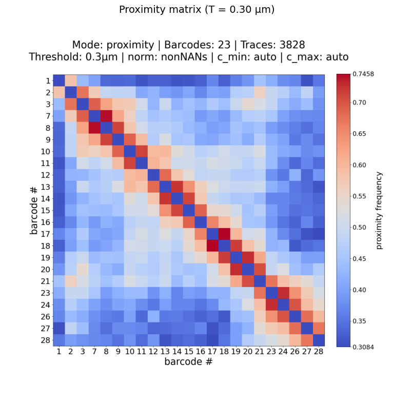
Plot: /home/devos/Documents/data_to_compare_pdx1/PDX1/plots/Fig_merged_traces_split_Matrix_PWDscMatrix_proximity_norm_T0.3_0.31-0.75.png

Example: median PWD matrix

!plot_him_matrix -M {sc_matrix} -B {barcodes} --mode median -O {data_path}/plots

Output path: /home/devos/Documents/data_to_compare_pdx1/PDX1/plots
$ Matrix loaded: /home/devos/Documents/data_to_compare_pdx1/PDX1/merged_traces_split_Matrix_PWDscMatrix.npy
$ Unique barcodes loaded: [1, 2, 3, 7, 8, 9, 10, 11, 12, 13, 14, 15, 16, 17, 18, 19, 20, 21, 23, 24, 26, 27, 28]
$ averaging method: median
/home/devos/Repo/traceratops/.venv/lib/python3.11/site-packages/numpy/lib/_nanfunctions_impl.py:1215: RuntimeWarning: All-NaN slice encountered
  return fnb._ureduce(a, func=_nanmedian, keepdims=keepdims,
Output data: /home/devos/Documents/data_to_compare_pdx1/PDX1/plots/Fig_merged_traces_split_Matrix_PWDscMatrix_median_norm_0.20-0.40.npy

matches = sorted(glob.glob(f"{plots_path}/Fig_*_median_norm_*.png"))
if matches:
    img = mpimg.imread(matches[0])
    fig, ax = plt.subplots(figsize=(10, 8))
    ax.imshow(img)
    ax.axis('off')
    ax.set_title("PWD Median matrix", fontsize=14)
    plt.tight_layout()
    plt.show()
    print(f"Plot: {matches[0]}")

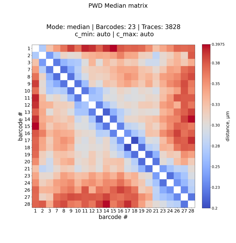
Plot: /home/devos/Documents/data_to_compare_pdx1/PDX1/plots/Fig_merged_traces_split_Matrix_PWDscMatrix_median_norm_0.20-0.40.png

Summary

Workflow

trace file (.ecsv)
       │
       ▼
trace_to_matrix              →  5 plots + 3 data files
       │
       ▼
plot_him_matrix (optional)   →  re-plot with custom options

Produced by trace_to_matrix

Plot	What it shows
*_HiMmatrix.png	Contact probability (proximity frequency)
*_PWDmatrixMedian.png	Pairwise distance — median
*_PWDmatrixKDE.png	Pairwise distance — KDE peak
*_Nmatrix.png	Data coverage (N measurements per pair)
*_PWDhistograms.png	Full distance distributions (all pairs)

Customization with plot_him_matrix

Use case	Command
Change distance threshold	--mode proximity -T 0.30
Median distance matrix	--mode median
KDE distance matrix	--mode KDE
Custom colormap	--c_map viridis --c_min 0.0 --c_max 0.5
Mask sparse bins	--nan_threshold 0.8
Triangular plot	--triangular --triangular_mode upper
PDF for publication	--plot_format pdf

Next: Tutorial 8 — Multiway Colocalization