Tutorial 8: Colocalization Analysis (2-way & 3-way)

Objective

Beyond pairwise distance matrices (Tutorial 7), chromatin tracing data allows us to ask: given a specific genomic locus (anchor), which other loci are physically close to it?

This tutorial covers two complementary analyses:

1. 2-way colocalization (plot_4m) — For a given anchor barcode, compute the frequency at which each other barcode is within a distance cutoff. Produces a 1D profile (4M plot).

2. 3-way colocalization (trace_3way_coloc) — For a given anchor barcode, compute the frequency at which pairs of other barcodes are both within the distance cutoff simultaneously. Produces a 2D heatmap.

Both scripts include bootstrapping to estimate statistical confidence (mean ± SEM).

Scientific context

• 2-way (4M): reveals which loci interact with a chosen viewpoint — analogous to 4C/Capture-C.

• 3-way: identifies higher-order contacts where 3 loci converge simultaneously — evidence for transcription factories, chromatin hubs, or phase-separated condensates.

Input

We use the Pdx1-positive trace file from Tutorial 6:

File	Description
Trace_3D_barcode_mask-mask0_ROI-16_Pdx1_Pdx1.ecsv	Traces inside the Pdx1 mask

import matplotlib.pyplot as plt
import matplotlib.image as mpimg
import glob

data_path = "/home/devos/Documents/data_to_compare_pdx1/PDX1"
input_trace = f"{data_path}/merged_traces_split.ecsv"

print(f"Input trace: {input_trace}")

Input trace: /home/devos/Documents/data_to_compare_pdx1/PDX1/merged_traces_split.ecsv

Step 1: 2-way colocalization with plot_4m

plot_4m computes, for a chosen anchor barcode, how frequently every other barcode is found within a distance cutoff. This is repeated over bootstrap iterations to obtain mean ± SEM.

The result is a 4M plot: a 1D profile where the X-axis is the barcode number and the Y-axis is the colocalization frequency with the anchor.

Parameters

Option	Default	Description
--input	—	Input trace file (ECSV)
--anchors	—	One or more anchor barcode numbers (space-separated)
--cutoff	0.2	Distance threshold in µm
--bootstrapping_cycles	10	Number of bootstrap iterations
--output	colocalization_plot.png	Base name for output plots
--x_min / --x_max	auto	X-axis range for the plot

# 2-way colocalization: anchor at barcode 10, distance cutoff 0.25 µm
!plot_4m --input {input_trace} --anchors 10 --cutoff 0.25 --bootstrapping_cycles 50 --output {data_path}/coloc_4m.png

$ Processing trace file: /home/devos/Documents/data_to_compare_pdx1/PDX1/merged_traces_split.ecsv
$ Importing table from pyHiM format
Successfully loaded trace table: /home/devos/Documents/data_to_compare_pdx1/PDX1/merged_traces_split.ecsv

$ Processing anchors: [10]

The output is saved as coloc_4m_anchor_10.png (the anchor ID is appended automatically).

plot_file = f"{data_path}/coloc_4m_anchor_10.png"

img = mpimg.imread(plot_file)
fig, ax = plt.subplots(figsize=(12, 5))
ax.imshow(img)
ax.axis('off')
ax.set_title("4M plot: colocalization with anchor barcode 10", fontsize=14)
plt.tight_layout()
plt.show()

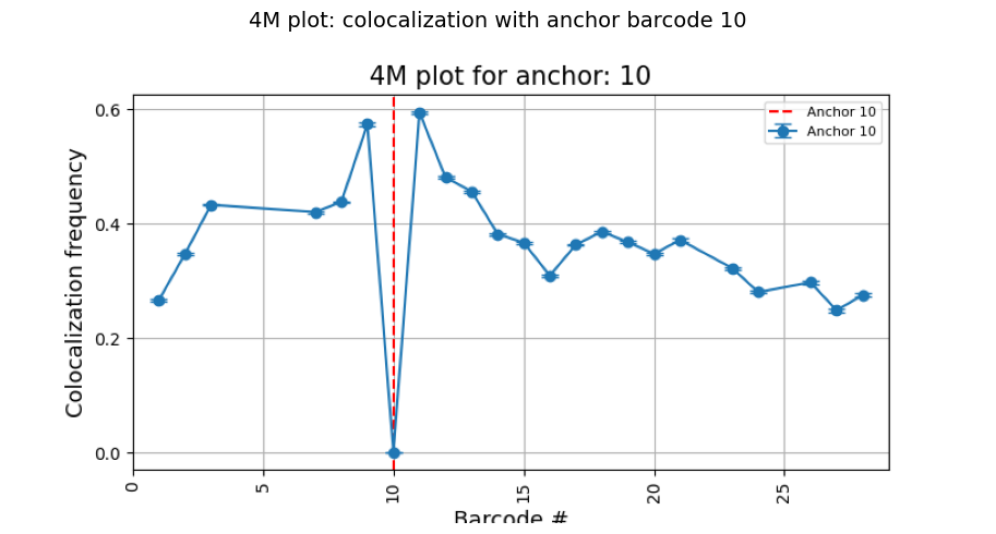
How to read the 4M plot:

• Each point is a barcode; the Y-value is the fraction of traces where that barcode is within 0.25 µm of the anchor.

• Error bars show the bootstrap SEM.

• The red dashed line marks the anchor barcode itself.

• Barcodes near the anchor on the genome (close barcode numbers) are expected to have higher frequencies.

• A barcode far on the genome but with high frequency suggests a long-range contact.

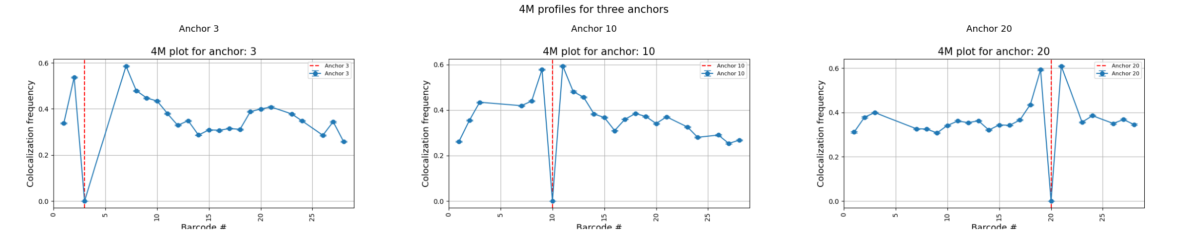
Multiple anchors

You can compute 4M profiles for several anchors in a single run. Each anchor produces its own plot.

# Multiple anchors in one run
!plot_4m --input {input_trace} --anchors 3 10 20 --cutoff 0.25 --bootstrapping_cycles 50 --output {data_path}/coloc_4m_multi.png

$ Processing trace file: /home/devos/Documents/data_to_compare_pdx1/PDX1/merged_traces_split.ecsv
$ Importing table from pyHiM format
Successfully loaded trace table: /home/devos/Documents/data_to_compare_pdx1/PDX1/merged_traces_split.ecsv

$ Processing anchors: [3, 10, 20]

# Display all anchor plots side by side
anchors = [3, 10, 20]
fig, axes = plt.subplots(1, 3, figsize=(24, 5))

for ax, anchor in zip(axes, anchors):
    plot_file = f"{data_path}/coloc_4m_multi_anchor_{anchor}.png"
    img = mpimg.imread(plot_file)
    ax.imshow(img)
    ax.axis('off')
    ax.set_title(f"Anchor {anchor}", fontsize=13)

fig.suptitle("4M profiles for three anchors", fontsize=15)
plt.tight_layout()
plt.show()

Step 2: 3-way colocalization with trace_3way_coloc

trace_3way_coloc extends the analysis to three-body contacts. Given an anchor barcode, it checks every pair of other barcodes (i, j) and asks: in what fraction of traces are anchor, i, and j all within the distance cutoff simultaneously?

The result is a symmetric heatmap where each cell (i, j) shows the 3-way colocalization frequency. A second heatmap shows the bootstrap SEM.

Parameters

Option	Default	Description
--input	—	Input trace file (ECSV)
--anchors	—	One or more anchor barcode numbers
--cutoff	0.2	Distance threshold in µm
--bootstrapping_cycles	10	Number of bootstrap iterations
--output	threeway_coloc_plot.png	Base name for output files
--vmin / --vmax	auto	Colormap range

# 3-way colocalization: anchor at barcode 10
!trace_3way_coloc --input {input_trace} --anchors 10 --cutoff 0.25 --bootstrapping_cycles 50 --output {data_path}/coloc_3way.png

>> Processing file: /home/devos/Documents/data_to_compare_pdx1/PDX1/merged_traces_split.ecsv
$ Importing table from pyHiM format
Successfully loaded trace table: /home/devos/Documents/data_to_compare_pdx1/PDX1/merged_traces_split.ecsv
Using distance cutoff: 0.25 µm
Performing 50 bootstrap iterations

Running analysis for anchor: 10
Saved three-way co-localization heatmap to: /home/devos/Documents/data_to_compare_pdx1/PDX1/coloc_3way_merged_traces_split_anchor_10
Saved SEM heatmap to: /home/devos/Documents/data_to_compare_pdx1/PDX1/coloc_3way_merged_traces_split_anchor_10_sem.png

This produces:

Output file	Description
coloc_3way_<trace_basename>_anchor_10.png	3-way frequency heatmap
coloc_3way_<trace_basename>_anchor_10.npy	Frequency matrix (NumPy)
coloc_3way_<trace_basename>_anchor_10_sem.png	Bootstrap SEM heatmap

# Find and display the 3-way heatmap (frequency and SEM)
freq_matches = sorted(glob.glob(f"{data_path}/coloc_3way_*_anchor_10.png"))
sem_matches = sorted(glob.glob(f"{data_path}/coloc_3way_*_anchor_10_sem.png"))

if freq_matches and sem_matches:
    fig, axes = plt.subplots(1, 2, figsize=(20, 8))

    img_freq = mpimg.imread(freq_matches[0])
    axes[0].imshow(img_freq)
    axes[0].axis('off')
    axes[0].set_title("3-way colocalization frequency", fontsize=14)

    img_sem = mpimg.imread(sem_matches[0])
    axes[1].imshow(img_sem)
    axes[1].axis('off')
    axes[1].set_title("Bootstrap SEM", fontsize=14)

    plt.tight_layout()
    plt.show()

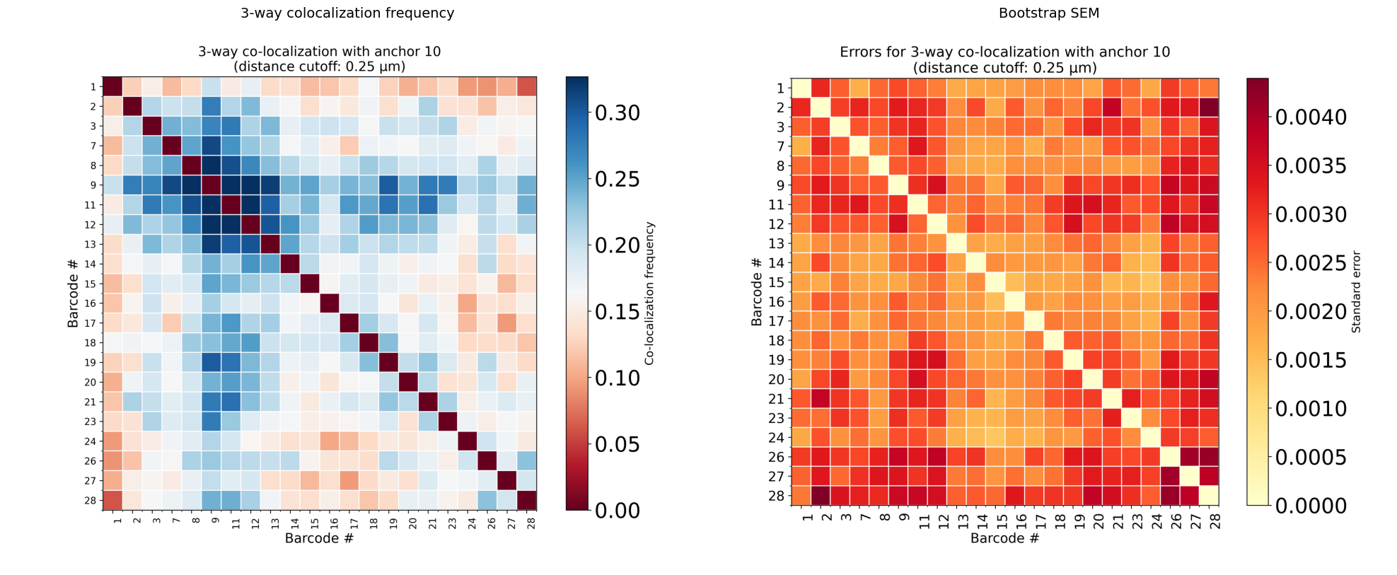
How to read the 3-way heatmap:

• Axes show barcode IDs (excluding the anchor).

• Cell (i, j) = fraction of traces where anchor, barcode i, and barcode j are all three within the distance cutoff.

• Black crosshair marks the anchor barcode position.

• High values off the diagonal reveal three-body hubs where three distant loci converge.

• The SEM heatmap helps identify which entries are statistically robust (low SEM).

Step 3: Varying the distance cutoff

The distance cutoff has a strong effect on colocalization frequencies. A small cutoff (e.g. 0.15 µm) captures only very tight contacts, while a larger one (e.g. 0.35 µm) includes more diffuse proximity. Try different values to see how the patterns change:

# Tight cutoff
plot_4m --input Trace.ecsv --anchors 10 --cutoff 0.15 --output coloc_tight.png

# Relaxed cutoff
plot_4m --input Trace.ecsv --anchors 10 --cutoff 0.35 --output coloc_relaxed.png

A robust interaction should be visible across a range of cutoffs.

Summary

Workflow

trace file (.ecsv)
       │
       ├─── plot_4m               →  1D profile (anchor vs each barcode)
       │
       └─── trace_3way_coloc      →  2D heatmap (anchor vs pairs) + SEM

Commands reference

# 2-way (4M profile)
plot_4m --input Trace.ecsv --anchors 10 --cutoff 0.25 --bootstrapping_cycles 50 --output 4m.png

# 3-way (heatmap)
trace_3way_coloc --input Trace.ecsv --anchors 10 --cutoff 0.25 --bootstrapping_cycles 50 --output 3way.png

Key differences

	plot_4m (2-way)	trace_3way_coloc (3-way)
Question	Is barcode X close to anchor?	Are barcodes X and Y both close to anchor?
Output	1D line plot	2D symmetric heatmap
Complexity	O(n) per trace	O(n²) per trace
Detects	Pairwise interactions	Higher-order hubs

Notes

• Bootstrap cycles: 10 is fast for exploration; use 100–1000 for publication.

• Multiple anchors: both scripts accept --anchors 3 10 20 to process several viewpoints in one run.

• Large datasets: 3-way analysis is computationally heavier than 2-way. For many barcodes, consider running on a filtered/split subset.

Next: Tutorial 9 — Compare datasets